0920
Computationally efficient depth-mapping scheme for human colliculi1Neuroscience, Rice University, Houston, TX, United States, 2Baylor College of Medicine, Houston, TX, United States, 3University of Chicago (NorthShore), Chicago, IL, United States
Synopsis
Determining depth in human colliculi is prone to errors due to its rapidly varying curvature. Thus, Euclidean definitions of depth fall short in describing the topography of deep collicular tissue. We developed a method of surface-based depth mapping that calculates a depth coordinate using an algebraic level-set method. We then generated kernels based on this level-set depth that sample functional data in a nonlinear trajectory with increasing depth. Using this method, we re-analyzed data on polar-angle representation of saccadic eye movements and were able to produce smoother laminar profiles that confirmed distinct depth-dependence of saccade-evoked activity.
Introduction
Human superior colliculus (SC) has a distinct laminar functional organization consisting of three major groups: superficial layers corresponding to visual stimulation, intermediate layers for oculomotor control, and deep layers for multisensory integration. Likewise, inferior colliculus has laminar segregation by auditory frequency. High-resolution functional MRI using sub-millimeter voxels allows for detailed laminar analysis of the functional topography of colliculi.
In the convoluted brain tissue, precisely specifying “depth” is difficult because of its variable curvature and thickness. Several methods developed to compute depth in cortex, including solutions of Laplace’s equation1 and equi-volume methods2, are computationally expensive to solve in a stable fashion. We offer a computationally simple surface-based approach based on an algebraic level-set scheme. We demonstrate its efficacy in distinguishing laminar profiles of activity within SC.
Methods
Acquisition & segmentation of anatomical images
For each of 4 subjects, we obtained high-resolution (0.7-mm voxels) T1-weighted volumes using an MP-RAGE sequence on a Siemens 3T scanner3. The brainstem tissue (BS) of each subject was segmented automatically using FreeSurfer4, manually using ITK-SNAP5, or both. A second manual segmentation was added to define the cerebral aqueduct (CA). From these two segmentations, we built surface models S1 and S2 enclosing BS and CA, respectively, by isovoxel triangulation, followed by refinement using a variational deformable surface approach6.
3D depth-mapping
From S1 and S2, we calculated signed distance functions d1 and d2, representing Euclidean point-to-triangle distances of each voxel to the nearest triangle of the corresponding mesh7. Sign was based on the segmentation. Thus, d1 is positive into BS, while d2 is positive within CA and negative in BS and surrounding CSF.
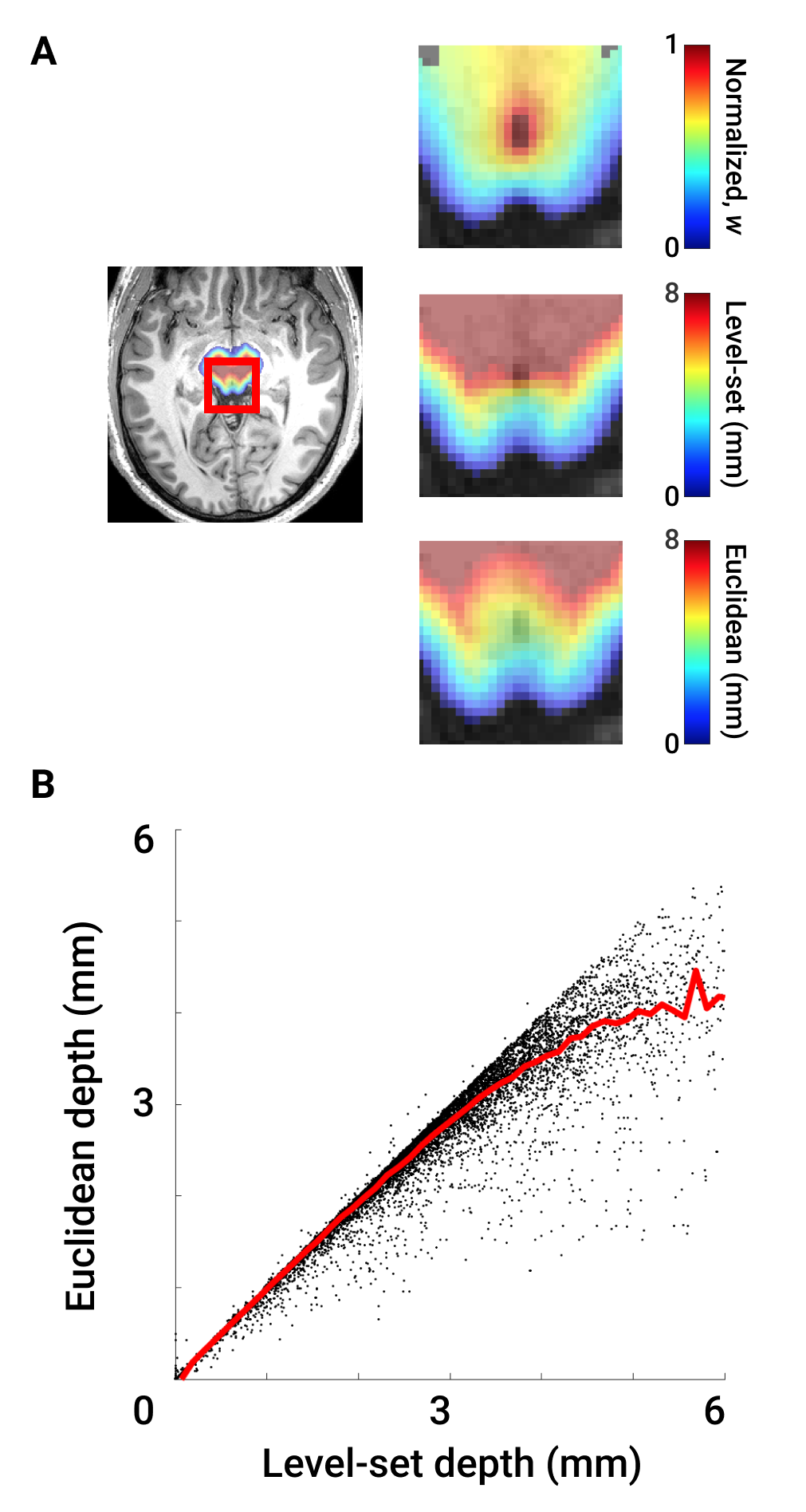
We then calculated a normalized depth coordinate, w, as a weighted sum of the signed distances using a level-set scheme8:
$$wd_{1}+ (1-w)d_{2}=0$$
w is zero on the brainstem surface and unity at the surface of CA. Likewise, w < 0 outside BS and w > 1 within CA (Fig 1A).
Generation of depth-averaging streamlines
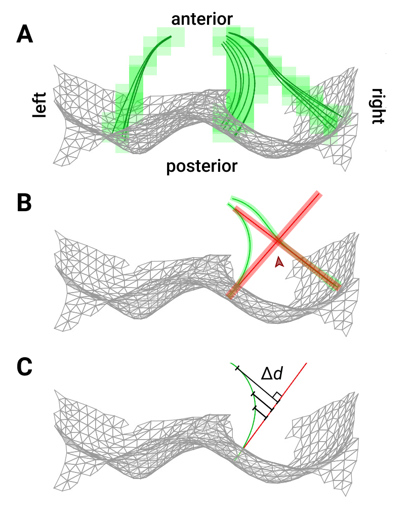
Treating w as a pseudopotential, we used its gradient to generate streamlines through BS that uniquely associate S1 and S2. ∇w was calculated by convolution with 5-point stencil kernels along each dimension. Then, we created streamlines originating at the vertices of S1 by ray tracing along ∇w (Fig 2A). Path distance along each streamline was regridded onto the volume using a Delaunay triangulation approach8 to create a non-Euclidean map of physical depth (Fig 1A).
Euclidean depth-analysis
For comparison, we utilized our earlier approach, which labeled each voxel of BS with its Euclidean nearest-neighbor distance to S1. Associations between surface vertices and deeper tissue were made using computational cylinders with central axes oriented along corresponding surface normals9 (Fig 2B).
Results
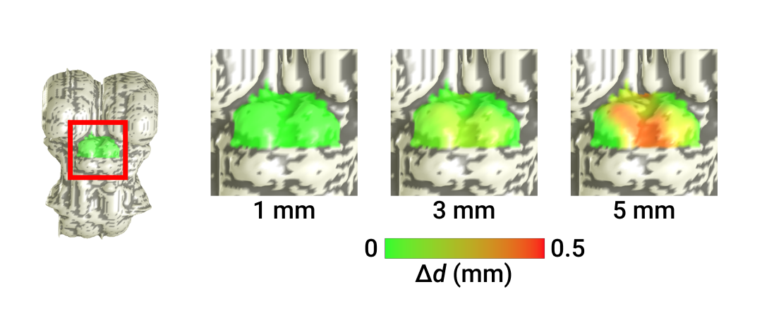
The relationship between Euclidean and non-Euclidean depth is sub-linear (Fig 1B), demonstrating non-linear deformation in deeper collicular tissue. Quantification of the deviation Δd (Fig 2C) between level-set and nearest-neighbor distance at increasing depths confirmed this observation. Further investigation into the spatial organization of Δd showed greatest error in inter-collicular regions, where surface normals point away from CA (Fig 3).
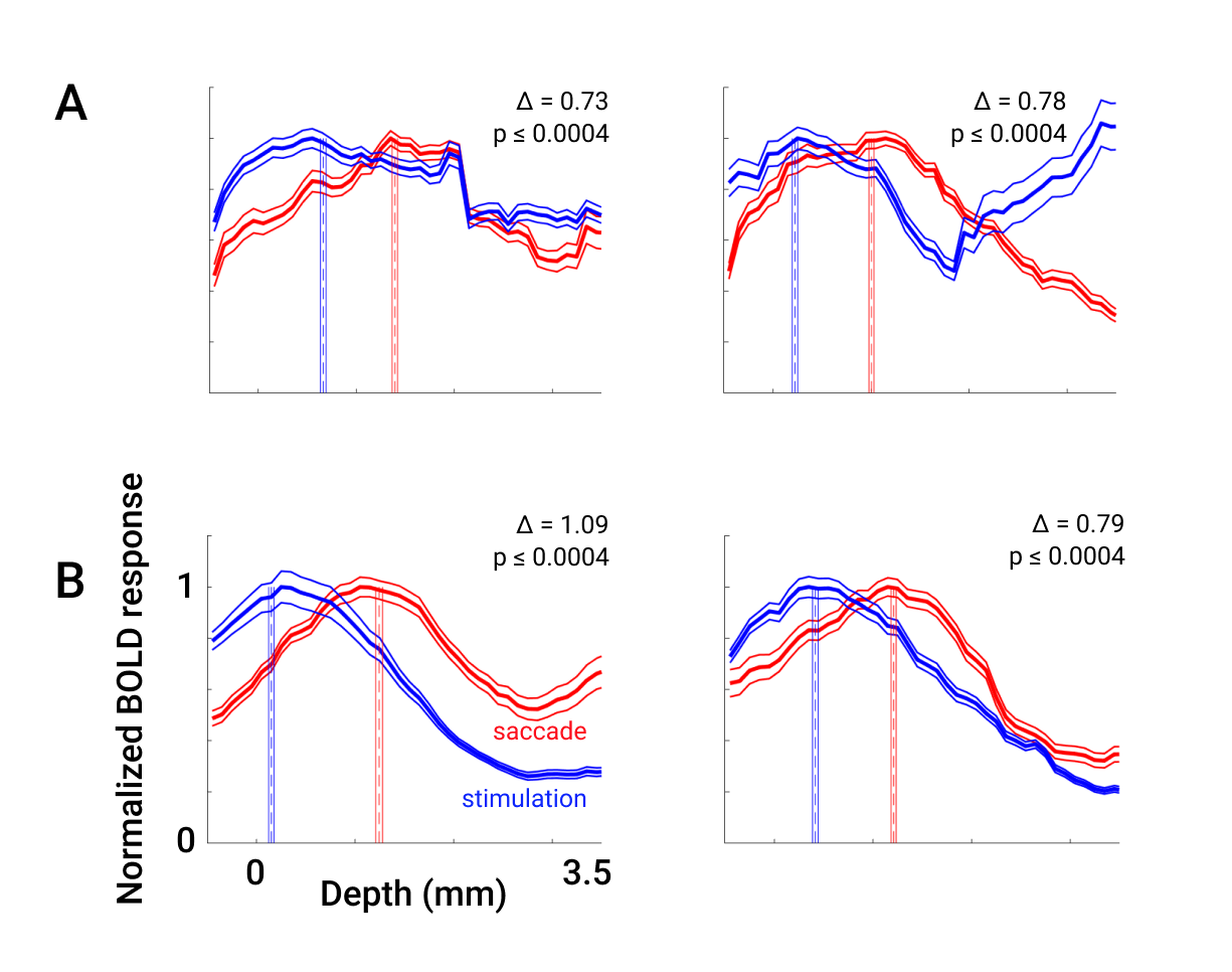
Additionally, we re-analyzed existing data on polar-angle representation of saccadic eye movements in SC3. Laminar profiles generated using level-set depth were able to qualitatively replicate the distinct offset between the peaks of stimulus- and saccade-evoked activity observed in profiles using Euclidean depth (Fig 3A,B). New profiles are smoother, have less variability, and show larger offsets between the two profiles with similarly high significance (new: left Δ = 1.09 mm, right Δ = 0.79 mm; old: left Δ = 0.72 mm, right Δ = 0.78 mm, all with p ≤ 0.0004).
Discussion
Our approach accommodates for the convoluted topography of the colliculi using a level-set method that logically relates all layers from superficial to deep tissue at all spatial locations on the brainstem surface. While depth-averaging approaches using nearest-neighbor associations are susceptible to oversampling deeper tissue and undersampling superficial tissue, the pseudopotential streamlines compress or expand along their depth, sampling regions of varying curvature more judiciously.
Compared to a Euclidean approach, major differences appear at depths > 3 mm. However, application of this method to measurement of laminar profiles of saccade- and stimulus-evoked activity resulted in increased depth differences despite the relatively superficial peaks of both profiles.
This method is easily applicable to cerebral cortex, using the gray-white interface as S1 and the pial surface as S2. Considering the large cortical surface area, a major merit of the algebraic level-set analysis is its computational simplicity compared to deformable-surface methods2,10.
Acknowledgements
No acknowledgement found.References
- Jones SE, Buchbinder BR, Aharon I. Three-dimensional mapping of cortical thickness using Laplace’s equation. Human Brain Mapping, 2000; 11(1):12-32.
- Waehnert MD, Dinse J, Weiss M, et al. Anatomically motivated modeling of cortical laminae. NeuroImage, 2014; 93(2):210-220.
- Savjani R, Katyal S, Halfen E, et al. Polar-angle representation of saccadic eye movements in human superior colliculus. NeuroImage, 2018; 171:199-208.
- Iglesias, JE, Van Leemput K, Bhatt P, et al. Bayesian segmentation of brainstem structures in MRI. NeuroImage, 2015; 113:184-195.
- Yushkevich PA, Piven J, Hazlett JC, et al. User-guided 3D active contour segmentation of anatomical structures: significantly improved efficiency and reliability. Neuroimage, 2006; 31(3):1116-1128.
- Xu G, Pan Q, Bajaj CL. Discrete surface modelling using partial differential equations. Computer Aided Geometric Design, 2006; 23(2):125-145.
- Eberly D. Distance between point and triangle in3D. Magic Software, 1999.
- Amidror I. Scattered data interpolation methods for electronic imaging systems: a survey. Journal of Electronic Imaging, 2002:11(2):157-176.
- Bajaj CL, Xu GL, Zhang Q. Bio-molecule surfaces construction via a higher-order level-set method. Journal of Computer Science and Technology, 2008; 23(6):1026-1036.
- Ress D, Glover GH, Liu J, et al. Laminar profiles of functional activity in the human brain. NeuroImage, 2007; 34(1):74-84.
Figures