0913
Dynamic functional connectivity and its relation to structural rich-club organisation1School of Aerospace, Mechanical and Mechatronic Engineering, The University of Sydney, Sydney, Australia, 2Melbourne School of Engineering, The University of Melbourne, Melbourne, Australia, 3Melbourne Neuropsychiatry Centre, The University of Melbourne, Melbourne, Australia, 4Sydney Imaging, The University of Sydney, Sydney, Australia, 5Florey Department of Neuroscience and Mental Health, The University of Melbourne, Melbourne, Australia
Synopsis
The relationship between static functional connectivity (FC) and structural connectivity (SC) has been long-recognised. More recently, functional connectivity has increasingly focused on the investigation of temporal variations of the BOLD fMRI signal; however, the role of SC on the observed FC fluctuations is not trivial or well understood. We show here that the structural rich-club organisation of the brain better describes the FC fluctuations than simply considering SC strength.
INTRODUCTION
The study of dynamic functional brain connectivity (dFC) has recently started to ask the question of the role of structural connectivity (SC) on the observed fluctuations within an fMRI session. While numerous studies revealed the strong dependencies between static FC and SC1, the relationship between the FC dynamics and SC, is not trivial or well known. Previous studies described this link at the level of functional network or with binary connections regarding FC, and in terms of number of anatomical connections or community partition regarding SC2. Using whole-brain weighted connectomes for both FC and SC, we showed here that the structural rich-club organisation of the brain better describes the dFC fluctuations than simply considering the SC strength.MATERIALS
Pre-processed functional (20min resting-state fMRI; 1200 volumes, TR=0.72s, 2mm isotropic resolution) and structural (b-values=0,1000, 2000, 3000 s/mm2, 90 directions/shell, 1.25mm isotropic resolution) data of 50 healthy subjects from the Human Connectome Project3 were used for this study – see 3–6 for details about acquisition and pre-processing steps. Subsequent diffusion MRI pre-processing was performed according to MRtrix recommendations (bias-field correction7, multi-shell multi-tissue CSD estimation8).
METHODS
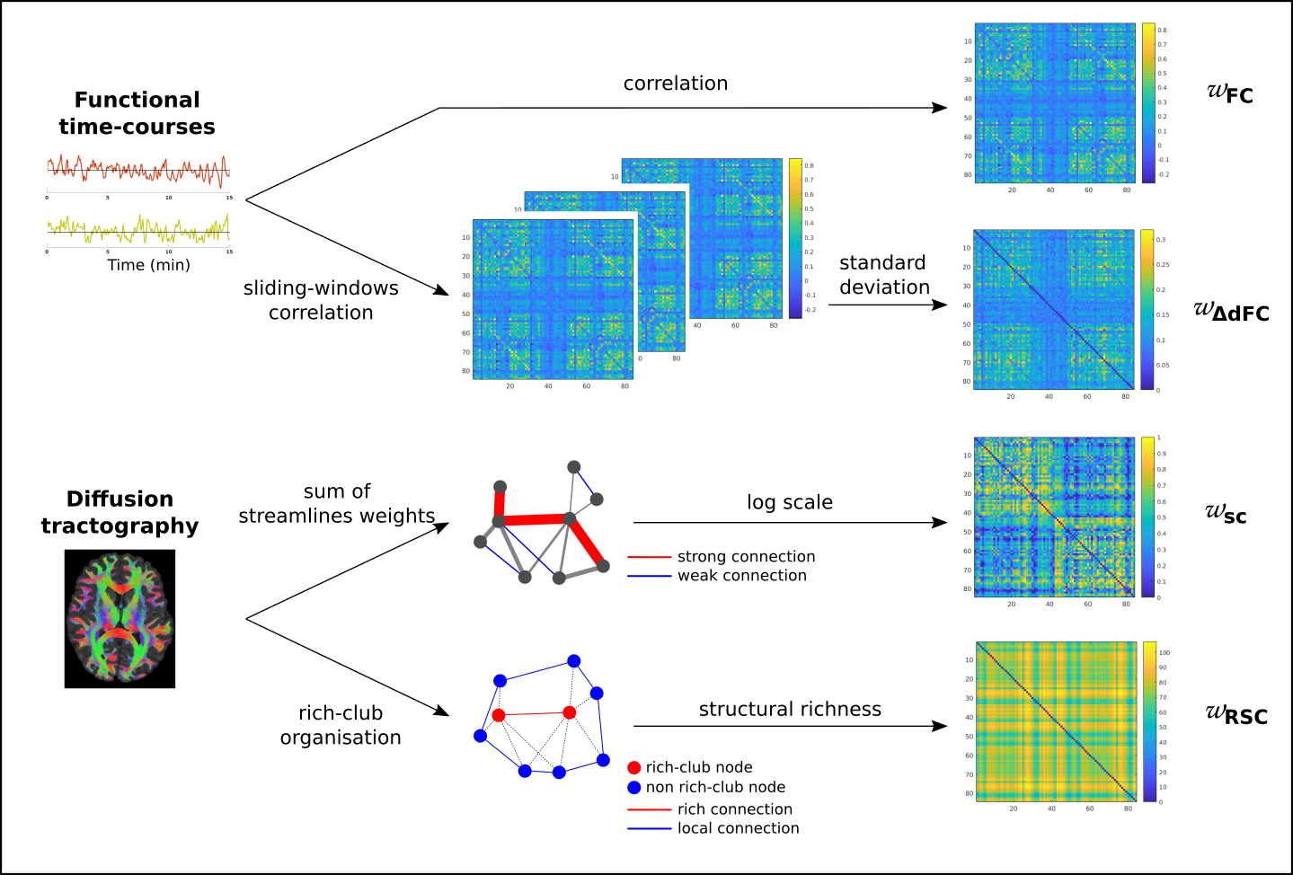
For each subject and for each edge of an 84-nodes network (FreeSurfer cortical parcellation9), we computed 4 values (see Fig. 1):
- Static FC (sFC): Pearson's correlation coefficients between mean time-course of each pair of regions, leading to a signed weight per edge (ωFC).
- Dynamic FC (dFC) was estimated with a sliding-window approach (94s tapered window, 1 TR step). Then, for each edge, the standard deviation over time (ωΔdFC) was computed.
- Structural weights were based on quantitative probabilistic streamlines tractography10–12: SC weights assigned to edges were generated by summing the streamlines weights connecting each pairs of regions11. The logarithm scale was used before a normalisation of theses weights (ωSC). Two ‘extreme’ groups were extracted from all edges as detailed in Fig. 1: the strongestSC connections group and the weakestSC connections group.
-
Structural rich-club
organisation
highlights highly connected nodes, the “rich-club
nodes”.13
We
quantified the rich-club effect by the weighted rich-club
coefficient14
based on the strength (computed as the sum of weights ωSC
of the node’s connections) of each node. By comparing with random
comparable networks, we kept 17 rich nodes, which was
the higher same number of rich-club nodes across subjects. Two types
of edges were defined15: richSC
connections (linking 2 rich-clubs) and localSC
connections (linking 2 non rich-clubs). Structural
richness
was calculated by adding the strength of the 2 nodes forming an edge
(ωRSC).
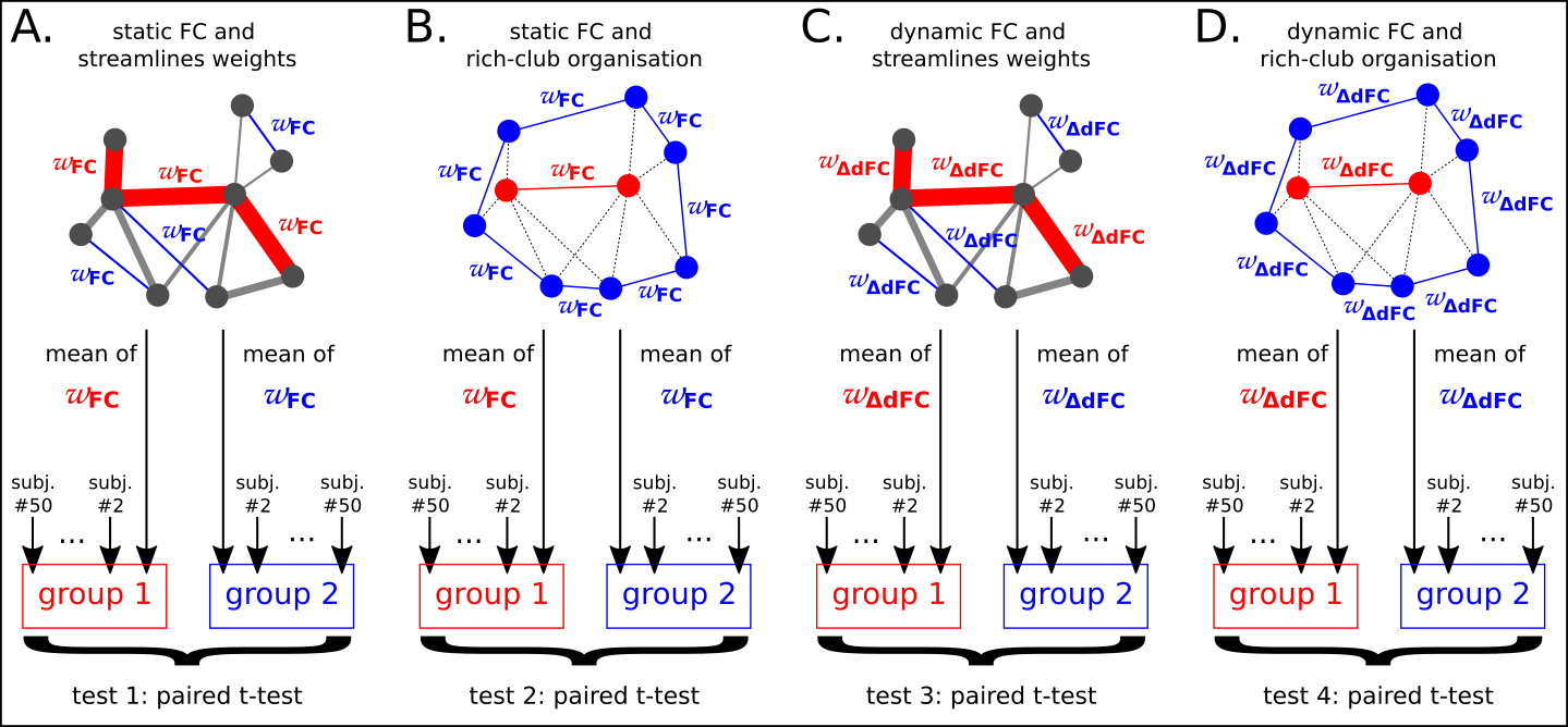
To evaluate which SC metric is the most suitable to describe dFC, we performed 4 comparisons: we aim to distinguish the strongestSC from the weakestSC and the richSC from the localSC from both a sFC perspective and a dFC perspective. It led to 4 comparisons that were assessed with paired sample t-tests as shown in Fig. 2.
In addition, we evaluated the statistical relationship between FC and SC with 4 correlations r(ωFC,ωSC), r(ωFC,ωRSC) , r(ωΔdFC,ωSC) , r(ωΔdFC,ωRSC).
RESULTS
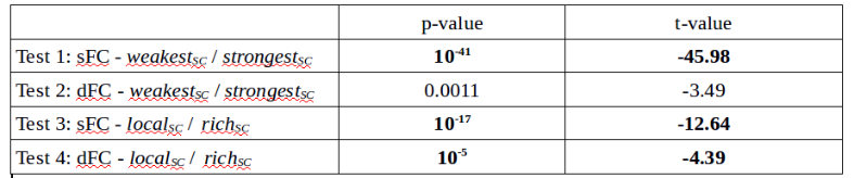
Table 1 shows that for static FC very low p-values were achieved revealing a strong difference between the richSC
and the localSC (p-values of 10-17) even more significant between the strongestSC
and the weakestSC
(p-value of 10-41). When associated with dynamic FC, a very low p-value (10-5) was achieved regarding the difference between the richSC
and the localSC and a low but higher one (0.0011) between the strongestSC
and the weakestSC. Negative t-values reveal lower FC fluctuations for localSC and weakestSC than for richSC and strongestSC.
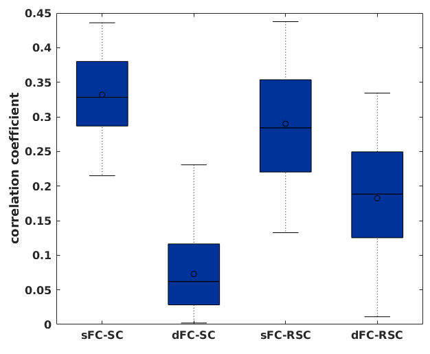
Fig. 3 shows lower correlation coefficients between dynamic FC and SC than between the 3 others comparisons.
DISCUSSION
We compared the rich edges vs. the local edges (topology of SC) and the strongest edges vs. weakest edges (strength of SC) in terms of their behaviour in sFC and dFC. As previously shown16, there is a strong relationship between sFC and SC; this relationship was found here to be more significant with the SC weight than with the rich-club classification. In contrast, our results showed that the rich-club classification better captures the dFC behaviour of the data than the weight of SC connections. One should consider studying (and inferring) dFC from the rich-club SC organisation rather than from direct SC matrices.CONCLUSION
While
the static FC is strongly
associated with the
number of anatomical connections, this study shows the important
influence of the
SC to other
areas (through the structural richness) when we study fluctuations of
FC. This
suggests that FC fluctuations between two areas depend more on their
importance in the overall organisation of the brain (structural
richness) than on their simple anatomical relationship (in terms of
structural connectivity).
Acknowledgements
We thank Dr. Oren Civier for pre-processing the structural data and Dr. Daniel Roquet for helpful comments.
This work was supported by funding from the National Health and Medical Research Council of Australia, the Australian Research Council, and the Melbourne Bioinformatics at the University of Melbourne, grant number UOM0048.
Data were provided by the Human Connectome Project, WU-Minn Consortium (Principal Investigators: David Van Essen and Kamil Ugurbil; 1U54MH091657) funded by the 16 NIH Institutes and Centers that support the NIH Blueprint for Neuroscience Research; and by the McDonnell Center for Systems Neuroscience at Washington University.
References
1. Zhu, D. et al. Fusing DTI and fMRI data: A survey of methods and applications. Neuroimage. 2014;102: 184–191.
2. Fukushima, M. et al. Structure-function relationships during segregated and integrated network states of human brain functional connectivity. Brain Struct. Funct. 2018;223:1091–1106.
3. Van Essen, D. C. et al. The WU-Minn Human Connectome Project: An overview. Neuroimage. 2013;80:62–79.
4. Van Essen, D. C. et al. The Human Connectome Project: A data acquisition perspective. Neuroimage. 2012;62:2222–2231.
5. Smith, S. M. et al. Resting-state fMRI in the Human Connectome Project. Neuroimage. 2013;80:144–168.
6. Glasser, M. F. et al. The minimal preprocessing pipelines for the Human Connectome Project. Neuroimage. 2013;80:105–124.
7. Tustison, N. J. et al. N4ITK: Improved N3 Bias Correction. IEEE Trans. Med. Imaging. 2010;29:1310–1320.
8. Jeurissen, B., Tournier, J.-D., Dhollander, T., Connelly, A. & Sijbers, J. Multi-tissue constrained spherical deconvolution for improved analysis of multi-shell diffusion MRI data. Neuroimage. 2014;103:411–426.
9. Desikan, R. S. et al. An automated labeling system for subdividing the human cerebral cortex on MRI scans into gyral based regions of interest. Neuroimage. 2006;31;968–980.
10. Smith, R. E., Tournier, J.-D., Calamante, F. & Connelly, A. Anatomically-constrained tractography: Improved diffusion MRI streamlines tractography through effective use of anatomical information. Neuroimage. 2012;62:1924–1938.
11. Smith, R. E., Tournier, J. D., Calamante, F. & Connelly, A. SIFT2: Enabling dense quantitative assessment of brain white matter connectivity using streamlines tractography. Neuroimage. 2015;119:338–351.
12. Smith, R. E., Tournier, J.-D., Calamante, F. & Connelly, A. The effects of SIFT on the reproducibility and biological accuracy of the structural connectome. Neuroimage. 2015;104:253–265.
13. van den Heuvel, M. P. & Sporns, O. Rich-Club Organization of the Human Connectome. J. Neurosci. 2011;31:15775–15786.
14. Opsahl, T., Colizza, V., Panzarasa, P. & Ramasco, J. J. Prominence and control: The weighted rich-club effect. Phys. Rev. Lett. 2008;101:1–4.
15. van den Heuvel, M. P., Kahn, R. S., Goni, J. & Sporns, O. High-cost, high-capacity backbone for global brain communication. Proc. Natl. Acad. Sci. 2012;109:11372–11377.
16. Honey, C. J. et al. Predicting human resting-state functional connectivity from structural connectivity. Proc. Natl. Acad. Sci. U. S. A. 2009;106:2035–40.
Figures