Synopsis

This work introduces a novel multivariate deconvolution method to blindly estimate neuronal-related -signal changes in multi-echo fMRI data without prior knowledge of their timings. In contrast to current voxel-based approaches, this algorithm simultaneously deconvolves all brain’s voxel time series and uses structured spatio-temporal regularization to improve the quality of the estimates. Besides, it employs stability selection procedures to overcome the selection of regularization parameters of the deconvolution problem. We evaluate its performance in multiple realistic simulations, showing its potential to blindly detect BOLD events in paradigms when no prior information can be obtained.

Introduction

Multi-echo (ME) fMRI collects several time-series per voxel at different echo times ($$$TE$$$) that can be utilized for increased BOLD sensitivity^[1,2], and/or enhanced denoising based on the linear dependence of BOLD fluctuations with $$$TE$$$^[3]. We have recently proposed a deconvolution algorithm for ME-fMRI data, named Multi-echo Sparse Paradigm Free Mapping (ME-SPFM), that blindly estimates voxelwise time-varying changes in the transverse relaxation ($$$\Delta R_2^*$$$) and the net magnetization ($$$\Delta S_0 / \bar{S}_0$$$) without prior information about neuronal-related BOLD events^[4,5]. In this work, we follow up this work and propose Multivariate ME-SPFM (MvME-SPFM) that is able to operate at once in the entire brain by using $$$\mathcal{L}_1$$$- and $$$\mathcal{L}_{2,1}$$$-norm regularized estimators along with stability selection procedures. We evaluate its performance in simulations with varying noise levels and spatial configurations.

Methods

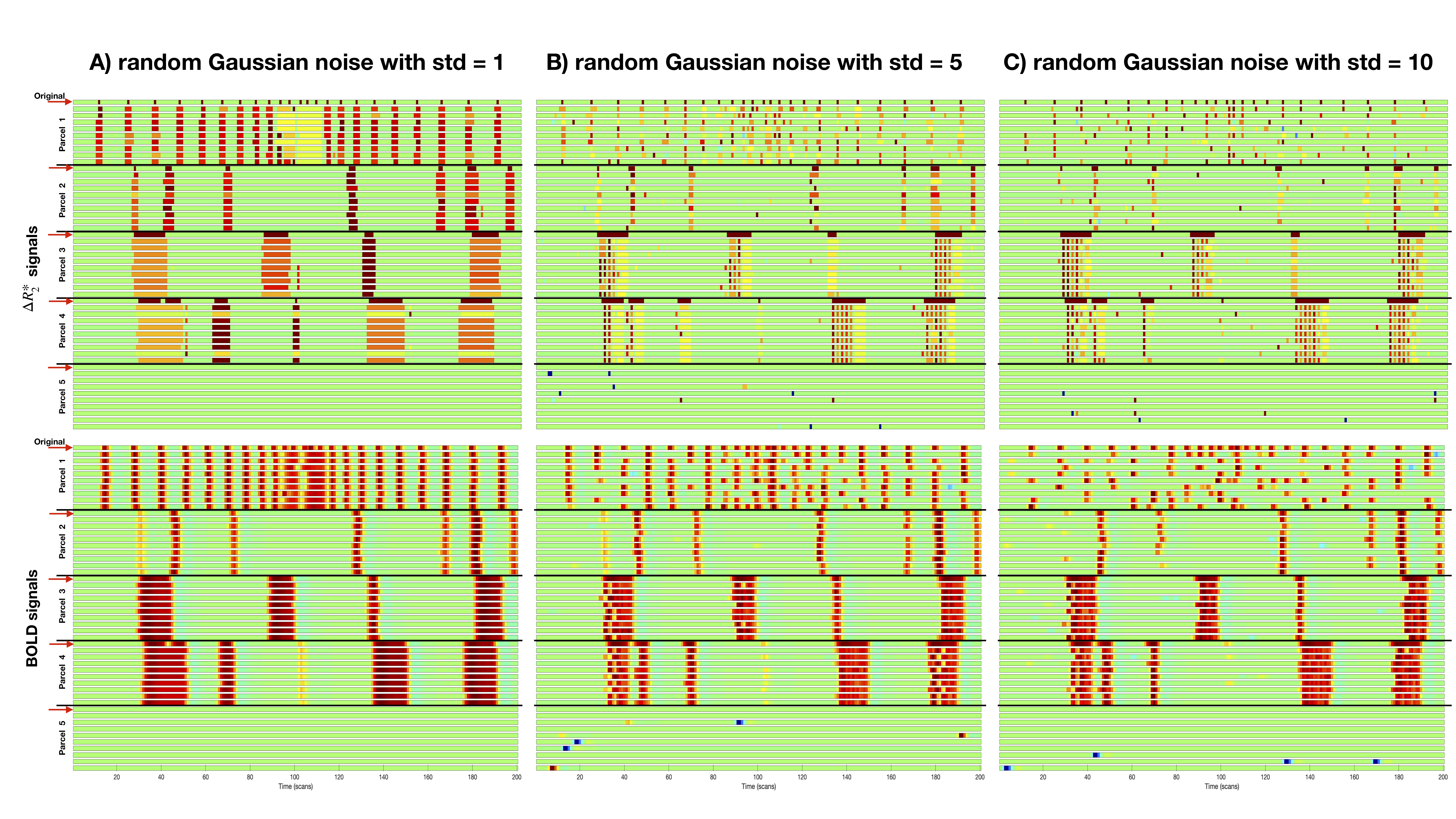
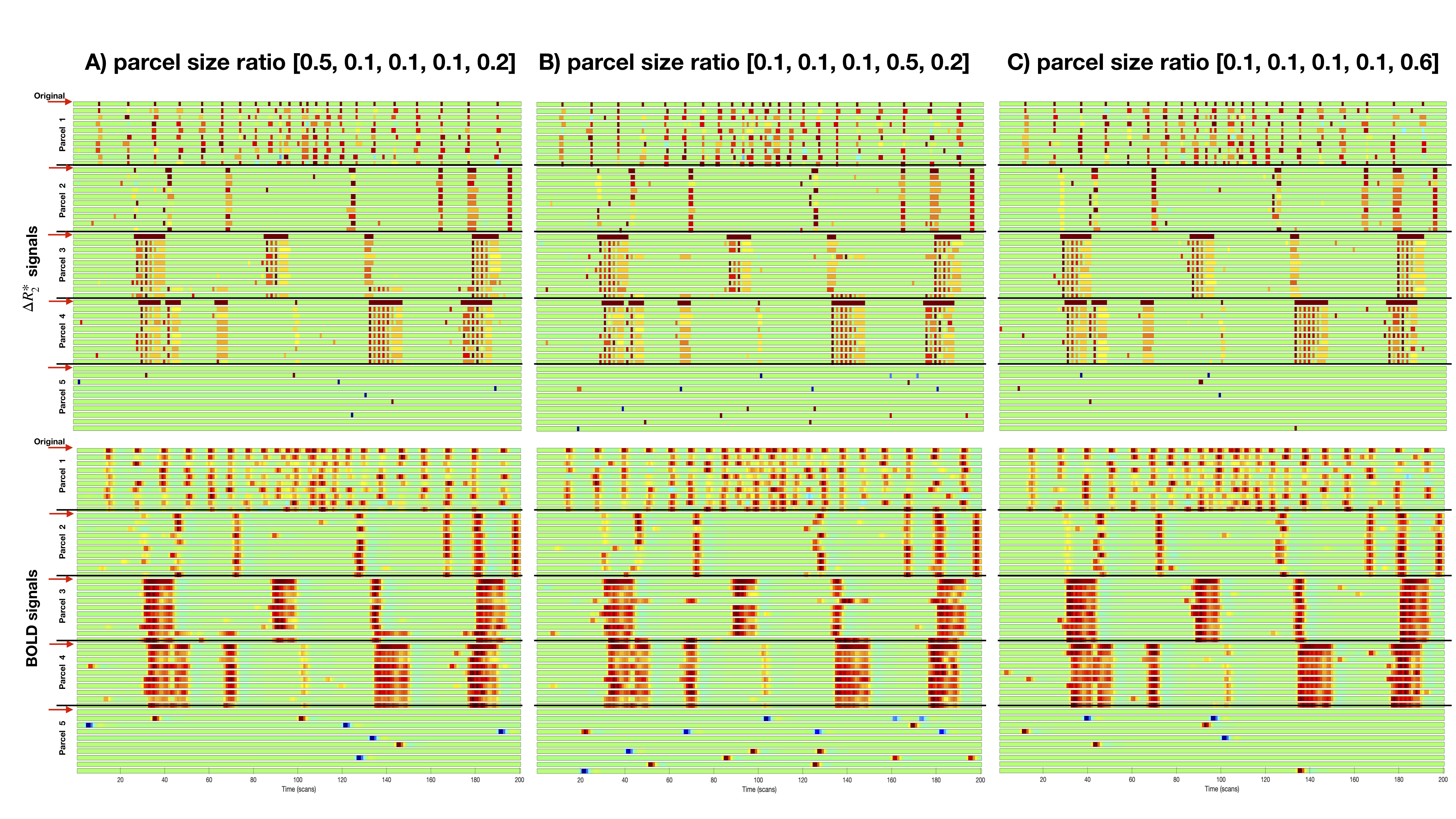
Data: A total of $$$V$$$=1500 voxels were simulated in 5 parcels ($$$L$$$=200 time-points, $$$TR$$$=2 sec.). Parcels 1-4 comprised neuronal-related $$$\Delta R_2^*$$$ signals from the Total Activation Toolbox^[6] that were convolved with the SPM canonical HRF to create BOLD signals, and then added random Gaussian noise (Figure 1B). Parcel 5 only included noise. The BOLD signals were linearly scaled by the corresponding $$$TE$$$s=15/35/55 ms^[3,4,5]. Different signal to noise ratios (SNR) and parcels' size ratios were simulated.

MvME-SPFM: Signal percentage changes (SPC) of a voxel fMRI time series at time $$$t$$$ and $$$TE_k$$$ can be described as:

$$y\left(t,TE_k\right)=-TE_k \Delta R_2^*\left(t\right)+\Delta \rho\left(t\right),$$

where $$$\Delta \rho \left(t\right)=\Delta S_0\left(t\right)/\bar{S}_0$$$. Neglecting $$$\Delta \rho\left(t\right)$$$, we propose to solve the following multivariate regularized least squares problem to deconvolve $$$\Delta R_2^*\left(t\right)$$$:

$$\hat{\textbf{X}} = \arg \min_{\textbf{X}} \|\textbf{Y}-\bar{\textbf{H}}\textbf{X}\|_2^2+\lambda \left( \tau \left| \textbf{X} \right|_1 + \left(1-\tau\right) \left|\textbf{X} \right|_{2,1} \right),$$

where $$$\textbf{Y}\in\mathbb{R}^{N_{TE}L \times V}$$$ denote the SPC signals of all echoes (rows) and voxels (columns), $$$\textbf{X}\in\mathbb{R}^{L \times V}$$$ denote the estimates of $$$\Delta R_2^*$$$, and $$$\bar{\textbf{H}}\in\mathbb{R}^{N_{TE}L \times L}$$$ comprises convolution matrices defined by the canonical HRF per echo, each scaled by its TE^[4,5]. The $$$\mathcal{L}_1$$$-norm (LASSO) $$$\left|\textbf{X}\right|_1=\sum_{t=1}^{L}\sum_{n=1}^V\left| \left(\Delta R_2^*\right)_{t,n}\right|$$$ promotes temporal sparsity of $$$\Delta R_2^*$$$ estimates, whereas the $$$\mathcal{L}_{2,1}$$$-norm (GROUP LASSO) $$$\left|\textbf{X}\right|_{2,1}=\sum_{t=1}^{L}\sum_{n=1}^V \left( \left|\left(\Delta R_2^*\right)_n\right|_{2}\right)_t$$$ promotes sparse groups of estimates of $$$\Delta R_2^*$$$ at time $$$t$$$ across voxels^[7]. The algorithm is solved with the Fast Iterative Shrinkage Thresholding Algorithm^[8]. The tradeoff parameter $$$\tau \left(0 \leq \tau \leq 1\right)$$$ is set to 0.75. Instead of selecting a fixed $$$\lambda$$$, we propose to solve the optimization problem in 100 subsamples (each with 60% of samples of the entire dataset) for a range of $$$\lambda$$$ (0.95-0.05*max($$$\lambda$$$)), and then compute the area under the curve (AUC) of the stability paths of each $$$\Delta R_2^*$$$ estimate^[9] (Figure 2). This yields an AUC time series per voxel. Next, AUC values are thresholded based on the 99th percentile of the AUC values of a region assumed without neuronal-related activity (parcel 5). For those values exceeding the threshold, unbiased $$$\Delta R_2^*$$$ estimates are finally obtained via least squares.

Results

Figure 2 illustrates the stability paths exhibit a clearer distinction between the curves for coefficients with $$$\Delta R_2^*\neq$$$0 and $$$\Delta R_2^*$$$=0 with decreasing noise, and differences are larger for parcels 2, 3 and 4 with long blocks and/or sparse event-related $$$\Delta R_2^*$$$-changes than parcel 1 with frequent brief $$$\Delta R_2^*$$$-changes. Likewise, higher AUC values are observed in the histogram of parcel 5 with increasing noise. Figure 3 demonstrates MvME-SPFM is able to blindly deconvolve $$$\Delta R_2^*$$$-changes at the times of the simulated neuronal-related events (noise with std(n)=5), and yields accurate estimates of BOLD signal changes particularly for parcels 2, 3 and 4, and barely detects false $$$\Delta R_2^*$$$-changes in parcel 5 (i.e. high specificity). Figure 4 shows the results for 9 random voxels of each parcel, illustrating the effect of the spatial regularization of the GROUP LASSO. BOLD estimates are more accurate than $$$\Delta R_2^*$$$-estimates that tend to exhibit discontinuities within long events and deteriorate with increasing noise. Figure 5 illustrates varying the ratio of parcels’ sizes does not considerably modify the performance of the algorithm.

Discussion and conclusions

Acknowledgements

References

[1] Posse, S., Wiese, S., Gembris, D. , Mathiak, K. , Kessler, C. , Grosse‐Ruyken, M. , Elghahwagi, B. , Richards, T. , Dager, S. R. and Kiselev, V. G. (1999). Enhancement of BOLD‐contrast sensitivity by single‐shot multi‐echo functional MR imaging. Magn. Reson. Med., 42: 87-97.

[2] Menon, R. S., Ogawa, S. , Tank, D. W. and Uǧurbil, K. (1993). 4 Tesla gradient recalled echo characteristics of photic stimulation‐induced signal changes in the human primary visual cortex. Magn. Reson. Med., 30: 380-386.

[3] Kundu, P., Inati, S.J., Evans, J.W., Luh, W.M. and Bandettini, P.A. (2012). Differentiating BOLD and non-BOLD signals in fMRI time series using multi-echo EPI. NeuroImage, 60: 1759-1770.

[4] Caballero-Gaudes, C., Bandettini, P.A. and Gonzalez-Castillo, J. (2018). Improved detection of neuronal-related BOLD events of unknown timing with Multi-Echo Sparse Paradigm Free Mapping. ISMRM 2018. Abstract #5463

[5] Gonzalez-Castillo, J., Caballero-Gaudes, C. and Bandettini, P.A. (2018). Quantitative deconvolution of neuronal-related BOLD events with Multi-Echo Sparse Free Paradigm Mapping. ISMRM 2018, Abstract #1124.

[6] Karahanoglu, F.I., Caballero-Gaudes, C., Lazeyras, F. and Van De Ville, D. (2013). Total activation: FMRI deconvolution through spatio-temporal regularization. NeuroImage, 73: 121-134.

[7] Gramfort A., Strohmeier D., Haueisen J., Hamalainen M. and Kowalski M. (2011) Functional Brain Imaging with M/EEG Using Structured Sparsity in Time-Frequency Dictionaries. In: Székely G., Hahn H.K. (eds) Information Processing in Medical Imaging. IPMI 2011. Lecture Notes in Computer Science, vol 6801. Springer, Berlin, Heidelberg

[8] Beck, A. and Teboulle, M. (2009). A Fast Iterative Shrinkage-Thresholding Algorithm for Linear Inverse Problems. SIAM Journal on Imaging Sciences 2:1,183-202

[9] Meinshausen N. and Bühlmann, P. (2010). Stability selection. J. R. Statist. Soc. B. 72: 417–473.