0817
Rapid open source prototyping of Magnetic Resonance Fingerprinting using Pulseq to enable multi-site two vendor studies1Columbia University MR research center, Columbia University, New York, NY, United States, 2Functional MRI Laboratory, University of Michigan, Ann Arbor, MI, United States
Synopsis
This work develops an open source package that allows for rapid prototyping of magnetic resonance fingerprinting (MRF) using Pulseq. In this work, an inversion recovery steady state free precession (IR-SSFP) sequence is designed in Pulseq. TR, flip angles, and TE are selected to achieve variations of contrast. The sequence was implemented, simulated, and applied on five health volunteer brain scans. The scan time of one subject for single slice sequence was 35 seconds. The data was sliding window reconstructed and matched with the simulated dictionary. The dictionary matching shows similar T1 and T2 results as reported in literature.
Purpose
To provide a complete open source package including dictionary simulation, sequence design, image reconstruction and dictionary matching that allows for vendor neutral, fast prototyping of magnetic resonance fingerprinting using Pulseq.Introduction
Pulseq is an open source tool that allows fast prototyping of pulse sequence in MATLAB. It currently supports three vendor hardware platforms including GE and Siemens [1]. Magnetic resonance fingerprinting is an approach that allows for simultaneous quantification of tissue properties [2] and hence is a significant tool to understand multi-site multi-vendor variability in a quantitative manner. However, a vendor-neutral tool is required to enable consistent implementations across platforms for meaningful comparisons. In this work, we develop that package to enable comparisons between two sites with two vendors.Method
The package is entirely written in MATLAB 2018a. Dictionary was generated based on Extended Phase Graph simulations for the chosen TR, TE and flip angles combinations. The pulse sequence was implemented using Pulseq package with following parameters: maximum gradient amplitude 32 mT/m, maximum slew rate 130 T/m/s, field of view 225 mm and matrix size 256x256, with a total of 1000 acquisition time points. The total scan time per slice sequence was 30 seconds. In vivo brain scans of five subjects were acquired on Siemens 3T scanner. The scans were performed using a 20-channel head coil. The collected data was then sliding window reconstructed using Michigan Image Reconstruction Toolbox (MIRT) for Non-Uniform Fast Fourier reconstruction of spiral k-space data. Three voxels representing Gray matter (GM), White Matter (WM) and CerebroSpinal Fluid (CSF) were selected from reconstructed image and their signal evolutions were plotted to verify with the dictionary signal evolutions. The resulting data was matched with the dictionary to provide values of T1, T2. The mean and standard deviation of white matter and gray matter for both T1 and T2 maps for the five subjects were calculated and compared. The mean was calculated for the pooled data of all the five subjects.Results
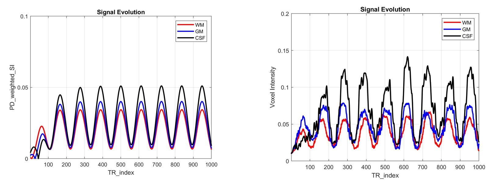
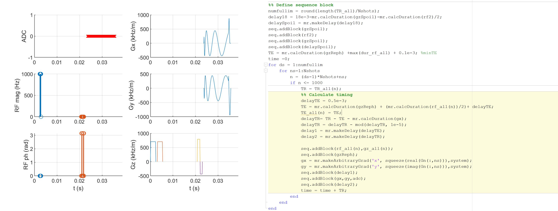
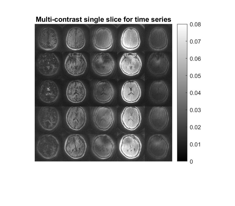
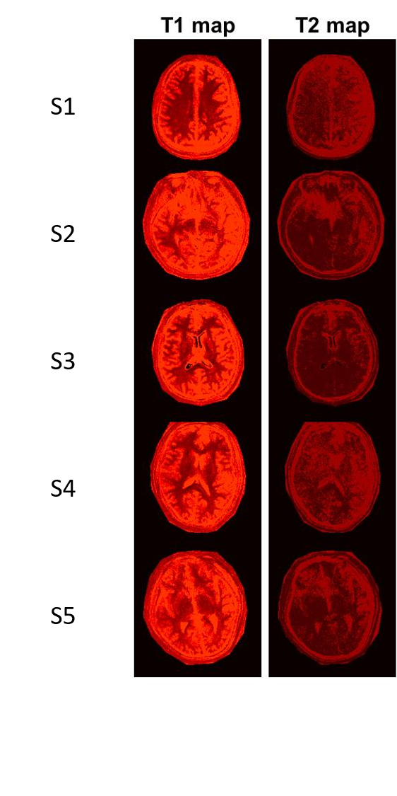
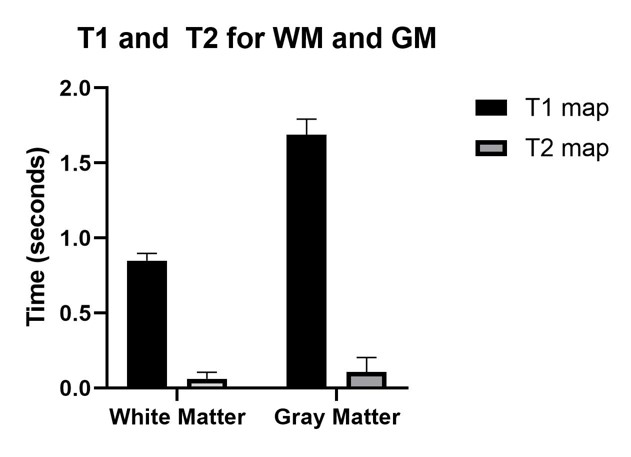
Figure 1 shows the signal evolution of dictionary entries and three voxels in reconstructed image representing WM, GM and CSF for all 1000 points. It can be observed that two signal evolutions are similar as expected. This verifies that the simulated dictionary agrees with the reconstructed image. Figure 2 shows the sequence plot and a screen capture of MATLAB Pulseq code used to generate the sequence. The sequence is generated by adding blocks of RF pulse, delay, gradients and etc. Figure 3 shows the reconstructed images at different time points for all five subjects. Different contrasts could be observed at different time points because of different flip angles and TR. At point 30, the image quality is poor due to not using full 48 shots of spirals. At point 80, white matter can be observed, which agrees with the signal evolution curve in Figure 1. Figure 4 shows the T1 and T2 maps after dictionary matching. The T2 mapping is less optimized than T1 mapping because higher degrees of flip angles are not included in current flip angle design. Figure 5 shows the mean and standard deviation of region of interest (ROI) of brain. The mean and standard deviation of T1 and T2 values of white matter and gray matter conform to the literature [3].Discussion and Conclusion
This package provides three benefits. Firstly, it is an open source package that includes a complete pipeline for prototyping MRF sequence. Secondly, by integrating with Pulseq, the package can be run on different vendor hardware including GE and Siemens scanners and the process time for MRF sequence prototyping iwould be greatly reduced. Ongoing and future work is to test our package on GE scanners and compare our results with Siemens scanners. To this end, the pulseq file has been translated to corresponding TOPPE files. Although Pulseq allows fast prototyping of pulse sequence on both vendors, the raw data collected from scanner are in different formats. This may require adjustments of current image reconstruction algorithms.Acknowledgements
No acknowledgement found.References
[1] Layton, K., Kroboth, S., Jia, F., Littin, S., Yu, H., Leupold, J., Nielsen, J., Stöcker, T. and Zaitsev, M. (2016). Pulseq: A rapid and hardware-independent pulse sequence prototyping framework. Magnetic Resonance in Medicine, 77(4), pp.1544-1552.
[2] Ma D, Gulani V, Seiberlich N, Liu K, Sunshine JL, Duerk JL, Griswold MA: Magnetic resonance fingerprinting. Nature 2013, 495:187–192.
[3] Wansapura, J., Holland, S., Dunn, R. and Ball, W. (1999). NMR relaxation times in the human brain at 3.0 tesla. Journal of Magnetic Resonance Imaging, 9(4), pp.531-538.
Figures