Synopsis

We introduce a method based on Gaussian Processes to rapidly acquire and reconstruct non-rigid motion fields of the human body directly from few points in k-space. Overall, the acquisition and processing time is less than 10 milliseconds for 3D applications leading to 100 Hz frame rate. Uncertainty quantification is also provided, making the method suitable for clinical real-time applications such as MR-guided radiation therapy.

Introduction

Theory

We present a probabilistic model which directly maps k-space data to the time dependent coefficients $$$\mathbf{y}^*_t$$$ of a motion field model (more on the motion model below). Such a probabilistic model is defined as a conditional distribution $$$P(\mathbf{y}^*_t|\mathbf{x}^*_t,\mathbf{X},\mathbf{Y})$$$, where $$$\mathbf{y}^*_t$$$ are the coefficients to be predicted at time $$$t$$$ and $$$\mathbf{x}^*_t$$$ is the on-line acquired k-space data. $$$\mathbf{X}$$$ and $$$\mathbf{Y}$$$ are training data. The mean, $$$\mu^y_t$$$ and standard deviation, $$$s^y_t$$$, of this probability distribution represent, respectively, the most likely motion coefficient and its uncertainty.

The central idea is to model $$$\mathbf{y}^*_t|\left\{\mathbf{x}^*_t,\mathbf{X},\mathbf{Y}\right\}$$$ as a Gaussian Process². Gaussian processes are very efficient when few training data are available and they provide closed form expressions for the prediction and its uncertainty. This leads to extremely fast computational schemes for the training as well as the prediction steps. In particular, $$$\mu^y_t$$$ and $$$s^y_t$$$ are given by

\begin{array}{ccl}\mu^{y}_t&=&\mathbf{k}^T_t(\mathbf{K}+\sigma^2\mathbf{I})^{-1}\mathbf{y}\\s^{y}_t&=&k(\mathbf{x}_t^*,\mathbf{x}_t^*)+\sigma^2-\mathbf{k}_t^T(\mathbf{K}+\sigma^2\mathbf{I})^{-1}\mathbf{k}_t\quad(1)\end{array}

where $$$\mathbf{K}$$$, $$$\mathbf{k}_t$$$ and $$$k(\mathbf{x}_t^*,\mathbf{x}_t^*)$$$ are quantities computed as kernels which depend on the training data $$$\mathbf{X}$$$ and the on-line data $$$\mathbf{x}^*_t$$$. The choice of kernel determines the type of underlying process. For smooth processes, square exponential kernels are typically used, which are characterized by two hyper-parameters: the length scale and the amplitude. The third hyper-parameter in the model is $$$\sigma$$$, which describes the uncertainty in the data. These three hyper-parameters are determined during training.

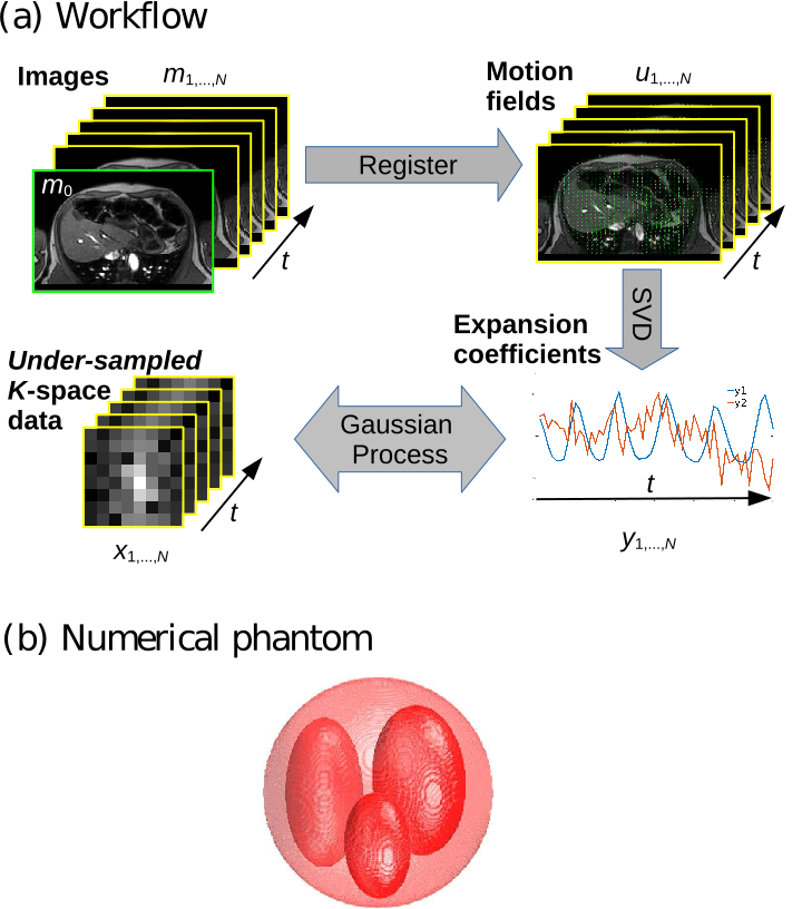
To obtain the motion model, motion fields $$$\vec{u}_t(\vec{r})$$$ are first generated by co-registering a set of cine-MRI images. An SVD is subsequently performed to derive a low-rank motion model³:

\begin{equation}\mathbf{u}_t=\mathbf{R}\mathbf{y}_t\end{equation}

for each snapshot. The data $$$\mathbf{Y}$$$ is assembled by concatenating all vectors $$$\mathbf{y}_t$$$.

Finally, the distribution of the predicted fields is also Gaussian and thus completely determined by its mean and covariance:

\begin{equation}\begin{array}{ccl}\boldsymbol{\mu}^{u}_t&=&\mathbf{R}\boldsymbol{\mu}^{y}_t\\ \mathbf{S}^{u}_t&=&\mathbf{RS}^{y}_t\mathbf{R}^T.\quad(2)\end{array}\end{equation}

Spatially-dependent confidence intervals are thus available.

Crucially, the operations in Eq. (1) and (2) and the acquisition of $$$\mathbf{x}_t$$$ take few milliseconds. The off-line training step takes few seconds. Figure 1(a) displays the workflow.

Methods

In these tests, we apply squared exponential kernel GP on the two principal components of the motion model.

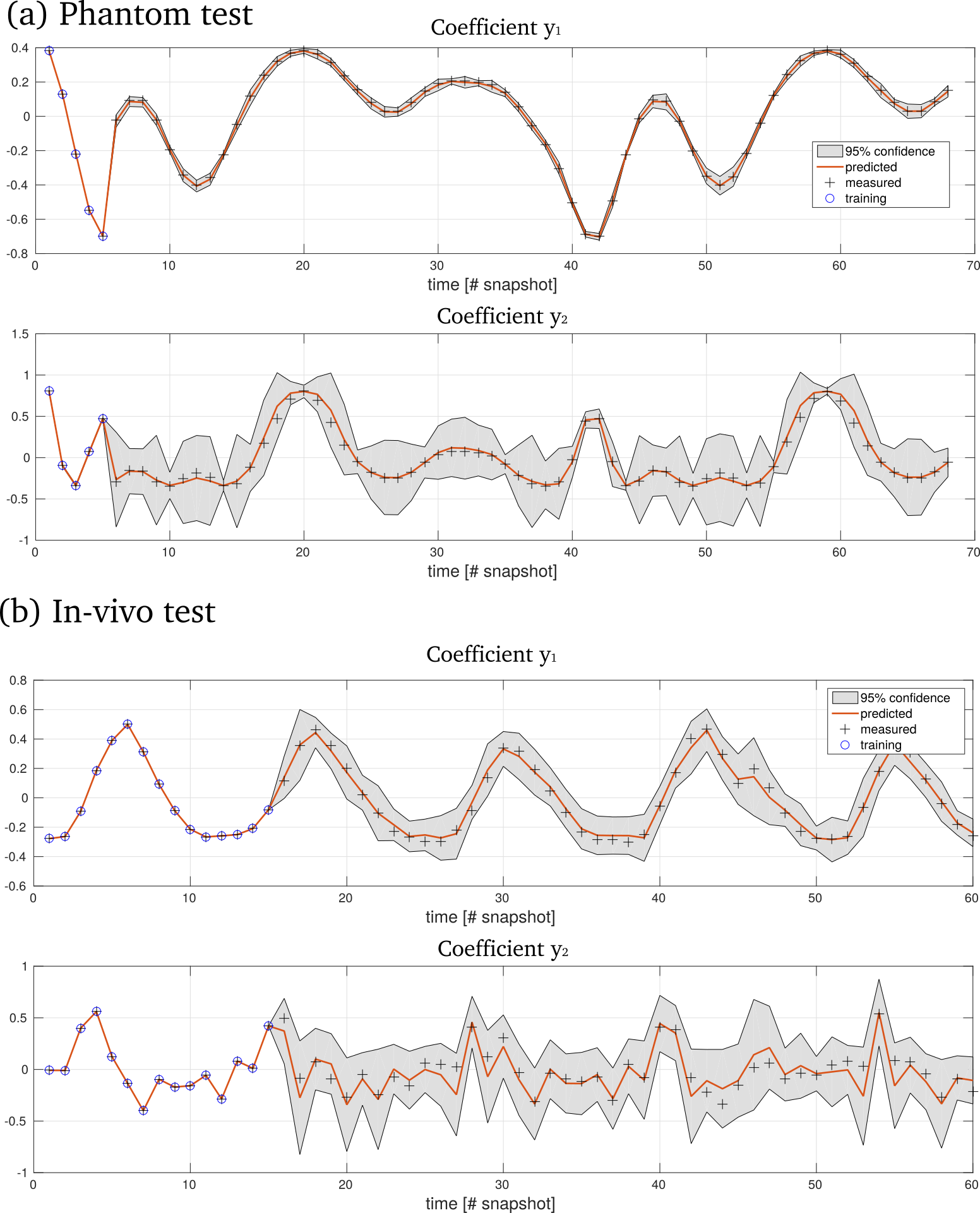
3D Phantom A $$$96\times96\times96$$$ spherical phantom with three ellipsoidal compartments is first considered (Fig. 1(b)). A nonlinear transformation is applied which deforms the object over 68 time points. As input $$$\mathbf{x}_t$$$, the central $$$4\times 4 \times 4$$$ k-space coefficients are taken and corrupted with noise (SNR = 20). For training, $$$N=5$$$ snapshots are considered.

2D In-vivo abdomen On a 1.5T Philips Ingenia scanner, we acquired two-dimensional $$$160\times 160 $$$ transverse cine-MRI images of the abdomen of a healthy volunteer during five breathing cycles (total: 60 snapshots). The 8-th image was taken as reference and all other snapshots were registered with the deformable optical-flow software RealTITracker⁴. Training and testing were performed on, respectively, the first 15 and remaining 45 snapshots. As input, the central $$$10\times10$$$ portion of the k-space data was used (retrospective undersampling).

Results

The reconstructed coefficients $$$\mu^y_t$$$ for the numerical phantom and in-vivo data are plotted in Fig. 2 and show good agreement with the actual coefficients. The gray-shaded area denotes the 95% confidence interval.

The true and reconstructed motion fields are shown in the animated Figures 3 (phantom) and 4 (in-vivo).

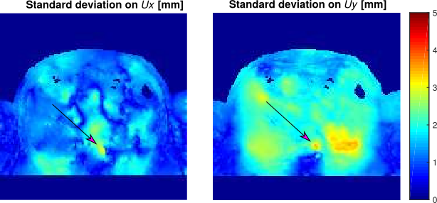
Figure 5 displays the reconstructed std maps for the in-vivo test. The uncertainty is higher in the regions corresponding to low signal intensity and the aorta. The latter is characterized by blood in-flow, which causes local disturbances (higher uncertainty) in the motion model.

Discussion and Conclusion

Our Gaussian process model recovers non-rigid motion fields directly from few k-space data points, leading to: (1) ultra-short acquisition times; (2) ultra-short processing times and (3) uncertainty estimation. For MR-guided radiation therapy, these three factors have crucial importance but can not be jointly addressed by state of the art techniques. The proposed GP framework can tackle these challenges at once.

Here, data was fully acquired and retrospectively undersampled to few k-space locations. These locations can be acquired by a spiral trajectory of few milliseconds leading to about 100 Hz frame rate. Such a real-time acquisition is being tested at the time of writing.

Acknowledgements

References

1. Crijns, S. P. M., B. W. Raaymakers, and J. J. W. Lagendijk. Proof of concept of MRI-guided tracked radiation delivery: tracking one-dimensional motion. Physics in Medicine \& Biology 57.23 (2012): 7863.
2. Rasmussen, C. E. and Williams, C. K. I. Gaussian processes for machine learning. MIT Press 2006.
3. Zhang, Qinghui, Alex Pevsner, Agung Hertanto, Yu‐Chi Hu, Kenneth E. Rosenzweig, C. Clifton Ling, and Gig S. Mageras. A patient‐specific respiratory model of anatomical motion for radiation treatment planning. Medical Physics 34, no. 12 (2007): 4772-4781.
4. Zachiu C., Denis de Senneville B., Moonen C. T. W., Ries M., A framework for the correction of slow physiological drifts during MR-guided HIFU therapies: Proof of concept, Medical Physics, 2015;42(7):4137-4148.