0793
Explaining current patterns on linear metallic implants during MRI exams using the transfer matrix.1Center for Image Sciences, UMC Utrecht, Utrecht, Netherlands, 2Department of Biomedical Engineering, Eindhoven University of Technology, Eindhoven, Netherlands
Synopsis
Currents induced on relatively(<20cm) short linear metallic implants typically occur in certain patterns. Knowledge of these patterns can help current monitoring and identification of hazardous exposure conditions. The transfer matrix (TM) of an implant predicts what patterns will appear. The eigenvalues of the TM indicate which modes are induced naturally. The projection of the eigenvectors onto realistic incident electric fields obtained from electromagnetic simulations explain which modes are likely and effectively excited. Over 80% of electric field distributions excite the first eigenmode of the investigated structures more efficiently. Moreover, all severe currents follow the pattern of this first eigenmode.
Introduction
MRI examinations of patients with (elongated) metallic implants pose a safety risk. The RF fields induce currents on the implants that cause temperature elevations at the tips of such implants1–3. The tip heating can be calculated from the incident RF electric field with an implant characteristic called the transfer function(TF)4. Recently, the TF concept has been extended to the transfer matrix(TM)5 allowing MR-based TF determination. This work will show the eigenmode spectrum of the TM contains valuable information on the most likely occurring current distributions on the implant. This information can help identify hazardous situations and critical incident electric fields. Knowledge of likely current patterns could furthermore benefit MR-based current monitoring6–8.
A simulation study is performed to investigate the eigenmodes of various elongated implant structures. This, in combination with a realistic collection of incident electric field distributions provides a framework to investigate the likelihood and shape of induced patterns.
Methods
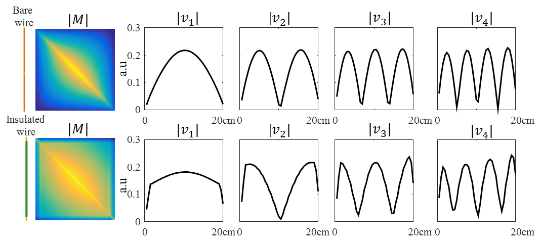
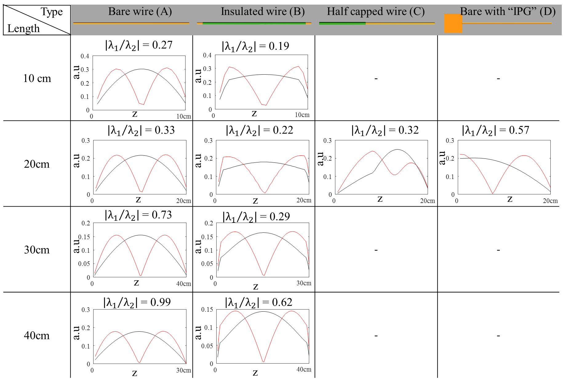
The TM,$$$\,M$$$, describes the one-dimensional current profile,$$$\,I_{ind}$$$, that will be induced on an implant exposed to an incident tangential one-dimensional electric field,$$$\,E_{inc}$$$, distribution through,$$$I_{ind}=ME_{inc}$$$. The TM is determined by FDTD electromagnetic simulations (Sim4Life, ZMT, Zurich, Switzerland). The implant is exposed to subsequently repositioned localized electric fields5 in a typical test medium9 ($$$\sigma=0.47$$$S/m,$$$\epsilon=78$$$). The TM is determined for the structures shown in figure 2.
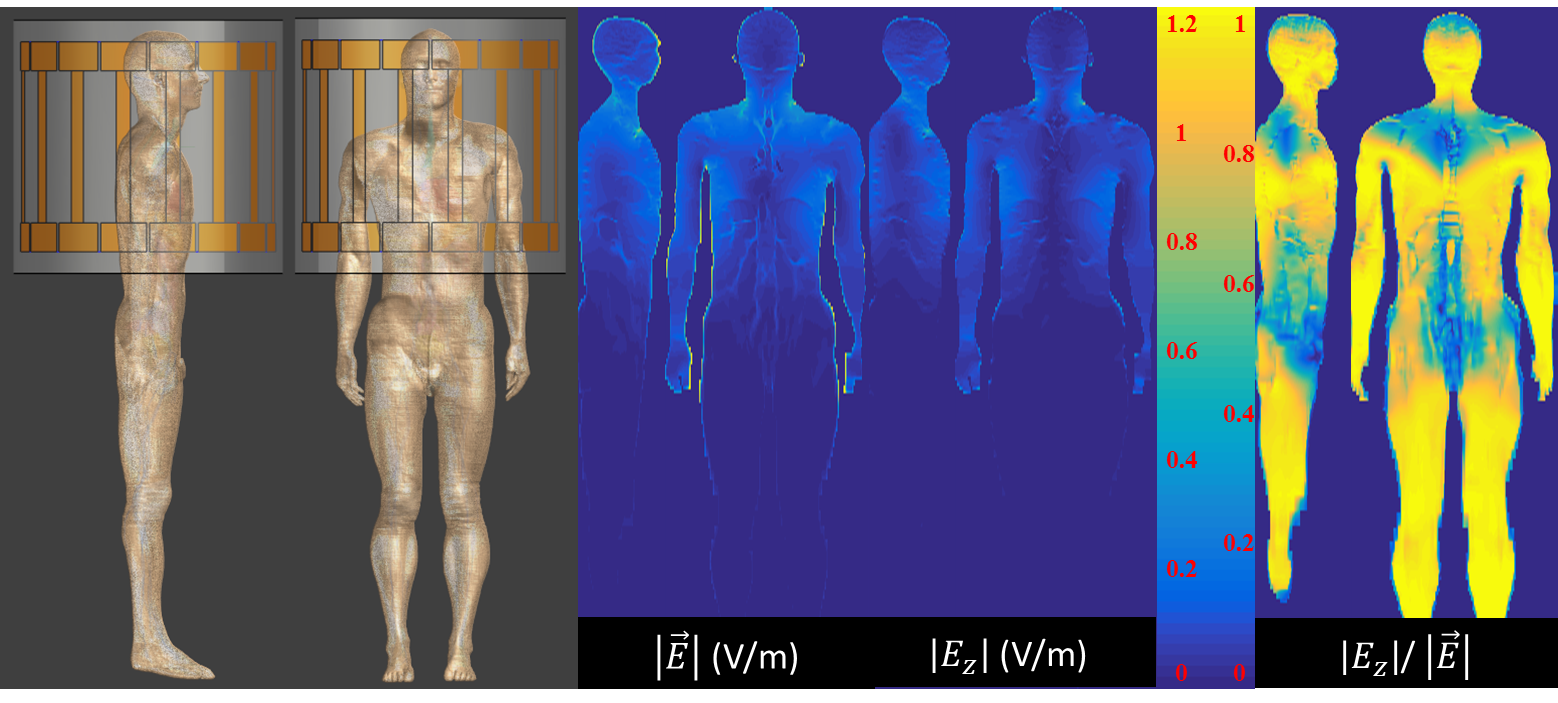
Possible realistic 1D electric field distributions are determined from a FDTD simulation of “Duke” from the Virtual Family10 in a 1.5T birdcage coil (figure 3). From the electric field distribution inside Duke all possible $$$E_{z,inc}$$$ exposures of 10cm, 20cm, 30cm and 40cm length are extracted. The wires are assumed to be z-oriented.
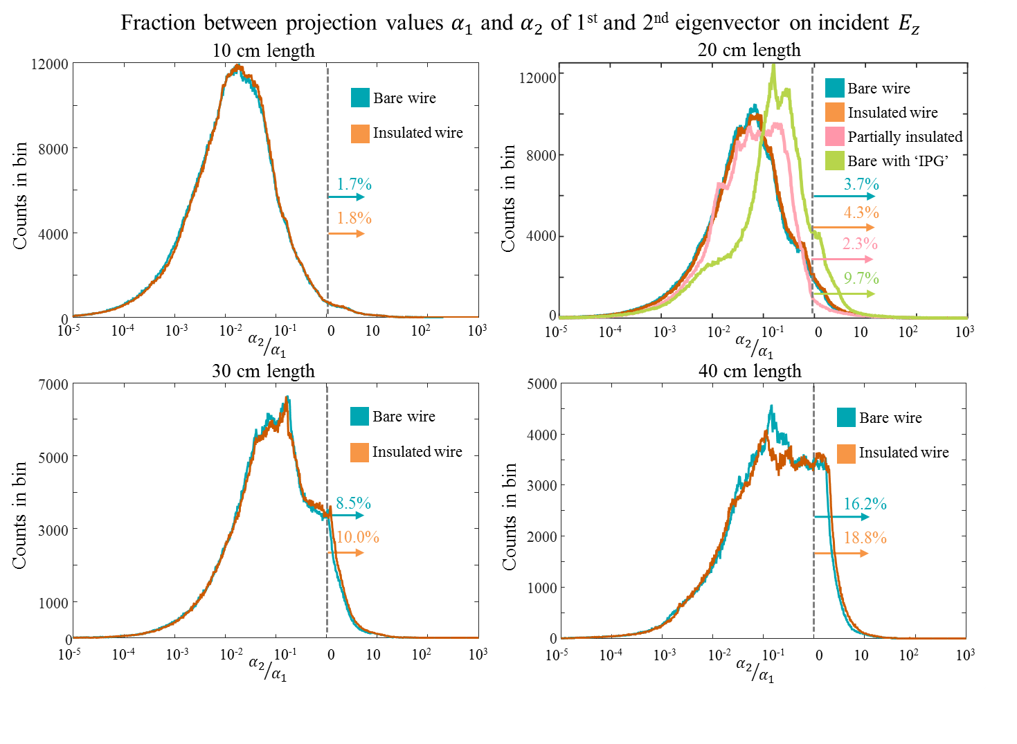
The eigenvalue distributions indicate that the first eigenvector will be induced most strongly. An $$$E_{inc}$$$ resembling this mode would be worst case. Nevertheless, the current pattern may resemble the second eigenvector if $$$E_{inc}$$$ predominantly projects onto this mode. To investigate how often this occurs, the $$$E_{z,inc}$$$ distributions from Duke are projected onto the eigenvectors. This identifies eigenmodes that are ‘excited’ more heavily. The higher the projection value, $$$\alpha_i$$$=$$$\frac{v_i\cdot E_{z,inc}}{||E_{z,inc}||_2}$$$, the more $$$E_{z,inc}$$$ induces this eigenmode,$$$\,v_i$$$. Secondly, the total induced currents are computed through a multiplication of the $$$E_{z,inc}$$$ distributions with the TM. The largest possible currents dominated by the first and second eigenmode are compared.
Results
Figure 1 shows two examples of TMs with their first 4 eigenvectors that resemble sine waves with decreasing wavelength. Figure 2 shows that the 1st eigenvalue is generally much bigger than the 2nd for shorter implants. This indicates that the implants support the first mode better than the others.
In total 2.83 million $$$E_{z,inc}$$$ of 10cm, 2.27 million $$$E_{z,inc}$$$ of 20cm, 1.85 million $$$E_{z,inc}$$$ of 30cm and 1.53 million $$$E_{z,inc}$$$ distributions of 40cm are extracted from the electric field inside Duke. The projection of these onto the 1st and 2nd eigenvector of the TM are denoted by $$$\alpha_1$$$ and $$$\alpha_2$$$. Figure 4 shows the $$$\frac{\alpha_2}{\alpha_1}$$$ histogram for the extracted collection of incident electric fields. The first eigenvector is excited more strongly for over 80% of $$$E_{z,inc}$$$ distributions.
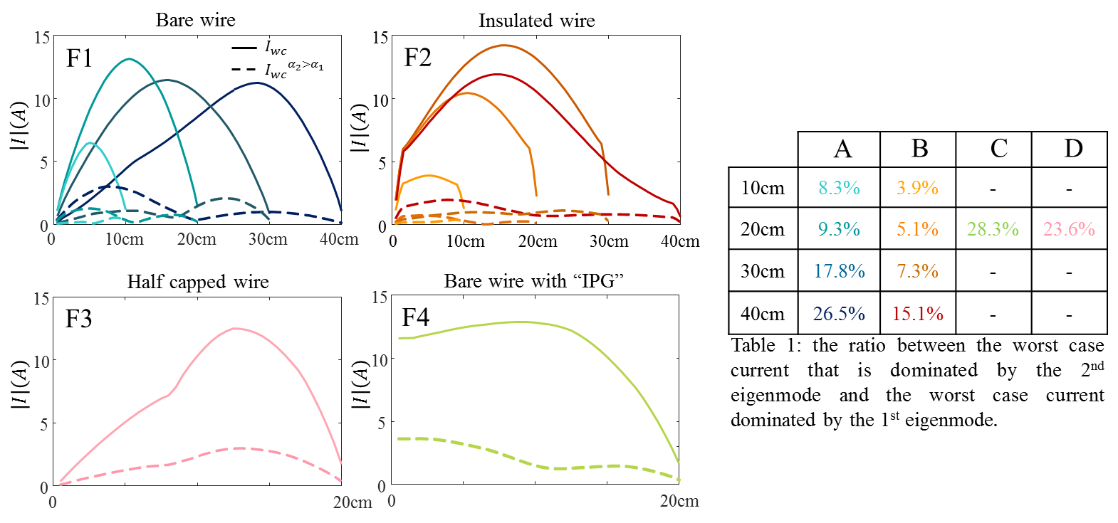
The contribution of each eigenvector to the currents computed from the $$$E_{z,inc}$$$ distributions by multiplication with the TM are calculated. In figure 5 the worst case currents dominated by the first and second eigenmode are displayed.
Discussion
The eigenvectors of the TM provide a basis set of modes to describe induced currents. Currents induced on an implant at 1.5T almost always appear in a pattern similar to the first dominant eigenvector. Which mode dominates depends on the length of the implant and the wavelength of the RF field in the medium, which is 44cm11.
Dominant eigenmodes have one antinode for implants investigated in this work (figure 2). Furthermore the first modes for all structures are excited more effectively by realistic $$$E_{z,inc}$$$ distributions. Figure 4 shows that over 80% of the potential $$$E_{z,inc}$$$ distributions induce the first eigenmode more effectively than the second.
Figure 5 shows that the worst case induced currents not dominated by the first eigenmode are much lower than the true maximal current. The contribution of each eigenvector to $$$I_{ind}$$$ is influenced by both the ability of the implant to support it and the effectiveness of $$$E_{z,inc}$$$ in exciting this specific mode.
Conclusion
The eigenvalues/vectors of the TM can be used to investigate the tendency for certain current patterns to appear. An analysis for four elongated implant structures of various lengths has shown that current patterns induced on smaller (<20cm) implants are dominated by a single eigenvector. To induce strong currents, this dominant eigenvector has to be excited more strongly than others, which happens for over 80% of realistic $$$E_{z,inc}$$$ distributions. The resultant current distributions, when significant, hence always resemble this dominant eigenvector.Acknowledgements
This project is funded by The Netherlands Organisation for Scientific Research (NWO) under project number: 15739.References
1. Konings MK, Bartels LW, Smits HFM, Bakker CJG. Heating around intravascular guidewires by resonating RF waves. J. Magn. Reson. Imaging 2000;12:79–85. doi: 10.1002/1522-2586(200007)12:1<79::AID-JMRI9>3.0.CO;2-T.
2. Luechinger R, Zeijlemaker VA, Pedersen EM, Mortensen P, Falk E, Duru F, Candinas R, Boesiger P. In vivo heating of pacemaker leads during magnetic resonance imaging. Eur. Heart J. 2005;26:376–383. doi: 10.1093/eurheartj/ehi009.
3. Nordbeck P, Fidler F, Weiss I, et al. Spatial distribution of RF-induced E-fields and implant heating in MRI. Magn. Reson. Med. 2008;60:312–319. doi: 10.1002/mrm.21475.
4. Park SM, Kamondetdacha R, Nyenhuis J a. Calculation of MRI-induced heating of an implanted medical lead wire with an electric field transfer function. J. Magn. Reson. Imaging 2007;26:1278–1285. doi: 10.1002/jmri.21159.
5. Tokaya JP, Raaijmakers AJ, Luijten PR, van den Berg CA, Janot Tokaya CP. MRI-based, wireless determination of the transfer function of a linear implant: Introduction of the transfer matrix. 2018:1–14. doi: 10.1002/mrm.27218.
6. van den Bosch MR, Moerland M a, Lagendijk JJW, Bartels LW, van den Berg C a T. New method to monitor RF safety in MRI-guided interventions based on RF induced image artefacts. Med. Phys. 2010;37:814–821. doi: 10.1118/1.3298006.
7. Griffin GH, Anderson KJT, Celik H, Wright G a. Safely assessing radiofrequency heating potential of conductive devices using image-based current measurements. Magn. Reson. Med. [Internet] 2015;73:427–441. doi: 10.1002/mrm.25103.
8. Griffin GH, Ramanan V, Barry J, Wright GA. Toward in vivo quantification of induced RF currents on long thin conductors. Magn. Reson. Med. 2018. doi: 10.1002/mrm.27195.
9. F2182-11a A. Standard Test Method for Measurement of Radio Frequency Induced Heating On or Near Passive Implants During Magnetic Resonance Imaging.
10. Christ A, Kainz W, Hahn EG, et al. The Virtual Family - Development of surface-based anatomical models of two adults and two children for dosimetric simulations. Phys. Med. Biol. 2010;55. doi: 10.1088/0031-9155/55/2/N01.
11. Nyenhuis JA., Park SM, Kamondetdacha R, Amjad A, Shellock FG, Rezai AR. MRI and implanted medical devices: Basic interactions with an emphasis on heating. IEEE Trans. Device Mater. Reliab. 2005;5:467–479. doi: 10.1109/TDMR.2005.859033.
Figures