0765
Efficient 3D low-discrepancy $$$k$$$-space sampling using highly adaptable Seiffert Spirals1Core-Facility Small Animal Imaging (CF-SANI), Ulm University, Ulm, Germany, 2Experimental Cardiovascular MRI (ExCaVI), Ulm University Medical Center, Ulm, Germany
Synopsis
The overall duration of acquiring a Nyquist sampled 3D dataset can be significantly shortened by enhancing the efficiency of $$$k$$$-space sampling. This can be achieved by increasing the coverage of $$$k$$$-space for every trajectory interleave. Further acceleration is possible by making use of advantageous undersampling properties.
This work presents a versatile 3D centre-out $$$k$$$-space trajectory, based on Jacobian elliptic functions (Seiffert's spiral). The trajectory leads to a low-discrepancy coverage of $$$k$$$-space, using a considerably reduced number of read-outs compared to other approaches. Such a coverage is achieved for any number of interleaves and therefore even single-shot trajectories can be constructed. Simulations and in-vivo studies compare Seiffert's spiral to the established 3D Cones approach.
Introduction
Fast volumetric imaging is usually achieved by undersampling in combination with GRAPPA, SENSE or Compressed Sensing (CS). General acceleration is possible by a rapid coverage of sampling $$$k$$$-space based on high $$$k$$$-space velocities and optimised sampling schemes, reducing coherent undersampling artefacts. But recent and efficient approaches such as FLORET1 or 3D Cones2 suffer from predominant sampling directions (symmetries) which cause disadvantageous undersampling properties. The presented approach reduces the occurrence of coherent artefacts by using adaptable Jacobian elliptic functions, while maintaining high $$$k$$$-space velocities, allowing further reductions in scan duration.Methods
One interleave of the trajectory is obtained by solving the problem of circling all meridians of a spherical surface at constant speed $$$v = \text{d}s/\text{d}t$$$ and angular velocity $$$\omega = \varphi/ t$$$ with $$$\varphi$$$ denoting the geographic longitude. Referring to Erdös3 a possible solution is given by Jacobi's elliptic functions cn($$$s|m$$$) and sn($$$s|m$$$). In cylindrical coordinates ($$$\rho,\varphi,z$$$), the trajectory (on a sphere) is parameterised by:
$$\begin{align}\varphi &= \kappa s \ \ \text{with} \ \ \kappa = \sqrt{m}, \\\rho &= \text{sn}(s|m), \ \ z = \text{cn}(s|m)\ \label{eq:fin}\end{align}$$
with $$$m$$$ being a parameter to account for gradient constraints. One centre-out $$$k$$$-space interleave is obtained by scaling the distance of each point w.r.t. the $$$k$$$-space centre linearly from 0 to $$$k_\text{max}$$$ while the length of the spiral corresponds to a certain read-out duration and resolution.
The generated Seiffert spiral is then rotated $$$N_\text{f}$$$ times such that the end point of each spiral is a Fibonacci point on the $$$k$$$-space sphere. The number of interleaves $$$N_\text{f}$$$ is calculated according to Nyquist's theorem.
Figure 1a) shows 250 arbitrarily selected interleaves of a trajectory and figure 1b) illustrates one-thousand Fibonacci points. The trajectory of figure 1a) represents the Seiffert spiral shown in green in figure 1c,d) in 3D and as $$$k_x$$$-$$$k_y$$$-plane projection.
The radial increment can be adapted to achieve different $$$k$$$-space densities. Exemplary, figure 1c,d) shows two different Seiffert spirals, with a quadratic (green) and square-root (orange) density modulation.
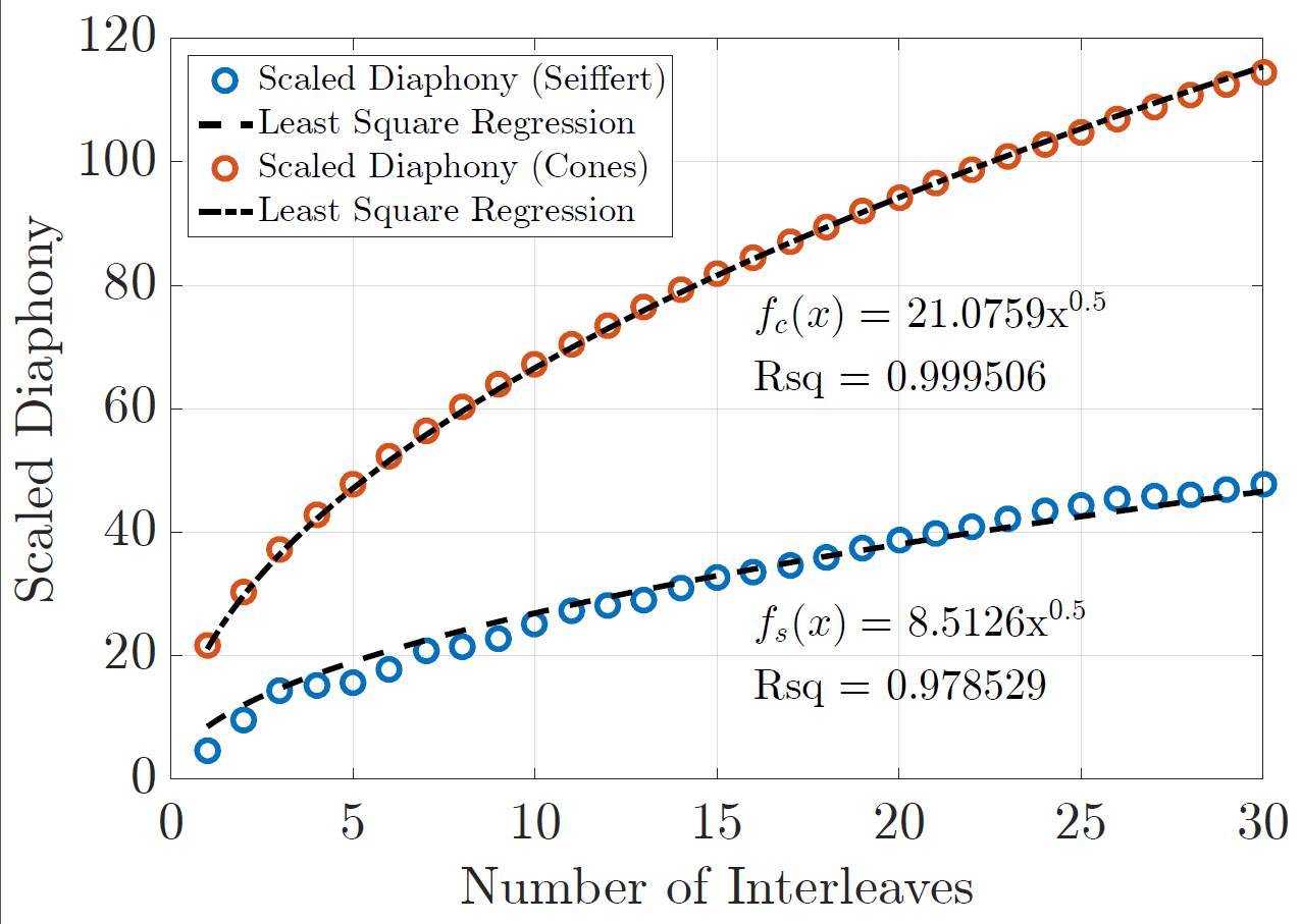
The distribution of $$$k$$$-space sampling points is analysed by the diaphony4. Figure 2 shows the calculated diaphony values for a considered number of interleaves for the 3D cones (red) and Seiffert approach (blue). Both trajectories were generated according to a resolution of 1.7 mm and a read-out duration of 3 ms.
The sampling point-spread functions for the Seiffert and Cones trajectories (4-fold undersampling) along the $$$x$$$ and $$$z$$$-direction are shown in figure 3.
In-vivo knee images with an isotropic resolution of 0.85 mm were acquired on a 3T wholebody MRI (Achieva 3T, Philips) using an 8-element SENSE knee coil. Undersampled images with a CS reconstruction are presented. All scan parameters are shown in figure 5. Eddy current effects were compensated using a mono-exponential model5 with a time constant of $$$\tau = 39$$$ $$$\mu$$$s.
The CS reconstructed images of the Seiffert approach correspond to a scan duration of $$$\approx\, 25$$$ s and to 22 times less excitations compared to a standard 3D cartesian acquisition and with a 20 % higher SNR compared to the Cones approach.
Results and Discussion
The scaled diaphony for the Seiffert approach is at least 2.35 times smaller, proving improved undersampling properties. Furthermore, the scaled diaphony of 100 arbitrarily selected interleaves of the Seiffert approach was at least 16 % smaller compared to the 3D Cones approach and at least 34 % smaller compared to a radial centre-out trajectory.
Along its symmetry axis ($$$z$$$), the 3D cones PSF shows clear spiral-like undersampling properties which remain coherent along all spatial directions. In contrast, the Seiffert spiral remains incoherent.
Fully sampled, 8-fold undersampled and CS reconstructed in-vivo knee images acquired with the Seiffert and 3D Cones approach are shown in figure 4. The Seiffert acquisition was accomplished using 20,000 excitations compared to 35,594 excitations for the 3D Cones scan. The Nyquist sampled Cones acquisition exhibits minor artefacts arising from gradient imperfections. The CS reconstruction is not capable of removing all coherent artefacts. In case of the Seiffert acquisition, all images show reduced degradation.
Conclusion
The presented approach based on Jacobian elliptic functions is capable of strictly reducing 3D scan durations due to its low-discrepancy generation algorithm which leads to an efficient coverage of $$$k$$$-space. Simulations and in-vivo images have shown clear advantages compared to the 3D Cones approach. A further decrease in scan duration is straightforward by exploiting the sequence's undersampling properties (random-noise-like) in combination with a CS reconstruction. Reconstruction methods using artificial neuronal networks such as machine- or deep learning may allow for even higher undersampling factors with no further degradation in image quality6.Acknowledgements
This project has received funding from the European Union's Horizon 2020 research and innovation programme under grant agreement No. 667192.
The authors thank the Ulm University Centre for Translational Imaging MoMAN for its support.
References
[1] J. G. Pipe, N. R. Zwart, E. A. Aboussouan, R. K. Robison, A. Devaraj and K. O. Johnson. A new design and rationale for 3D orthogonally oversampled k-space trajectories. Magn Reson Med. 66, 1303-1311, 2011.
[2] P. T. Gurney, B. A. Hargreaves and D. G. Nishimura. Design and analysis of a practical 3D cones trajectory. Magn Reson Med. 55, 575-582, 2006.
[3] P. Erdös. Spiraling the earth with CGJ Jacobi. Am J Phys. 68, 888--895, 2000.
[4] T. Speidel, J. Paul, S. Wundrak, V. Rasche. Quasi-Random Single-Point Imaging using Low-Discrepancy k-Space Sampling. IEEE Transactions on Medical Imaging. doi:10.1109/TMI.2017.2760919.
[5] I. C. Atkinson, A. Lu and K. R. Thulborn. Characterization and correction of system delays and eddy currents for MR imaging with ultrashort echo-time and time-varying gradients. Magn Reson Med. 62, 532-537. 2009.
[6] J. Schlemper, J. Caballero, J. V. Hajnal, A. N. Price and D. Rueckert. A deep cascade of convolutional neural networks for dynamic MR image reconstruction. IEEE Trans Med Imag. 37, 491-503. 2018.
Figures