0703
Quantitative Transport Mapping (QTM) of the Kidney using a Microvascular Network Approximation1Weill Medical College of Cornell University, New York, NY, United States, 2Cornell University, Ithaca, NY, United States
Synopsis
The blood flow quantification is of great importance in the diagnosis of many diseases. The current blood flow quantification methods are mainly based on the Kety’s method, which highly replies on the practically unmeasurable arterial input function (AIF). To void using the AIF as an input, we propose quantitative transport mapping (
Introduction
Perfusion imaging, the assessment of blood flow in small vessels and capillaries, is important for managing various diseases, including stroke, heart attack, and cancer. Current Kety model based methods require the identification of an arterial input function (AIF)1,2. However, the AIF is generally unmeasurable and usually assumed to be the same for the whole organ, which is biophysically inaccurate2. Here, we proposed a new method, called quantitative transport mapping (QTM), that characterizes the blood flow by reconstructing a blood velocity field from time-resolved tracer concentration data3,4. Using an approximate microvasculature for the kidney, it is shown that the velocity field can be used to estimate renal blood flow (RBF).Theory
$$$\hspace{1cm}{\bf\text{1.Biophysical model for QTM}}\hspace{5mm}$$$QTM reconstructs a blood velocity field$$$\,{\bf u}({\bf r})\,$$$ from tracer concentration data $$$c({\bf r},t)\,$$$according to the local mass conservation law. Assuming that the velocity$$$\,{\bf u}({\bf r})\,$$$is constant in time, the Fokker-Planck equation holds:
$$\frac{\partial c}{\partial c}=-\nabla\cdot(c{\bf u})-\gamma c+\nabla\cdot(D\nabla c),\hspace{3cm}(1)$$
where$$$\,\gamma\,$$$is the concentration decay rate and$$$\,D\,$$$the diffusion coefficient. Eq.1 describes the convection, decay, and diffusion effects of the tracer in the blood microvasculature. The values of$$$\,\gamma\,$$$and$$$\,D\,$$$depend on the tracer type. In this study we assume $$$\,D=0\,$$$ and $$$\gamma=1/T_1$$$ when using arterial spin labeling (ASL).
$$$\hspace{1cm}{\bf\text{2.Voxelization of QTM model}}\hspace{5mm}$$$Because the voxel size is much larger than the typical size of the micro vessels, Eq.1 should be integrated over a voxel before fitting. For a a voxel location$$$\,{\boldsymbol\xi}=(\xi_x,\xi_y,\xi_z)\,$$$ we obtain
$$J(C({\boldsymbol \xi},t), M^R,M^A,M^S,U,V,W)=0,\hspace{3cm}(2)$$
with
$$\hspace{-7cm}J=\frac{C({\boldsymbol\xi},t)-C({\boldsymbol\xi},t-\delta_t)}{\delta_t}+\lambda C({\boldsymbol\xi},t)$$
$$\hspace{-2cm}+\frac{C({\boldsymbol \xi},t)M^R({\boldsymbol \xi})U({\boldsymbol \xi})-C(\xi_x-1,\xi_y,\xi_z)M^R(\xi_x-1,\xi_y,\xi_z)U(\xi_x-1,\xi_y,\xi_z)}{V_m({\boldsymbol\xi})}$$
$$+\frac{C({\boldsymbol \xi},t)M^A({\boldsymbol \xi})V({\boldsymbol \xi})-C(\xi_x,\xi_y-1,\xi_z)M^A(\xi_x,\xi_y-1,\xi_z)V(\xi_x,\xi_y-1,\xi_z)}{V_m({\boldsymbol\xi})}$$
$$\hspace{-2cm}+\frac{C({\boldsymbol \xi},t)M^S({\boldsymbol \xi})U({\boldsymbol \xi})-C(\xi_x,\xi_y,\xi_z-1)M^S(\xi_x,\xi_y,\xi_z-1)W(\xi_x,\xi_y,\xi_z-1)}{V_m({\boldsymbol\xi})},$$
where$$$\,C({\boldsymbol\xi})\,$$$is the concentration averaged over the voxel and $$$V_m({\boldsymbol\xi})$$$ the blood volume, $$$M^R,\,M^A\,$$$and$$$\,M^S\,$$$the total vessel areas that intersects with the Right, Anterior, and Superior voxel surfaces, respectively. The latter four parameters are called the microvasculatural parameters (MP) below. $$${\bf U}=(U,V,W)\,$$$is the apparent blood velocity field to be reconstructed.
$$$\hspace{1cm}{\bf\text{3.Inverse problem of QTM}}\hspace{5mm}$$$The inverse problem of QTM is to solve for$$$\,{\bf U}\,$$$in Eq.2 using 4D data$$$\,C,$$$5
$$\min_{\bf U}\sum_{k=1}^N\|J(C({\boldsymbol \xi},t^k),M^R,M^A,M^S,U,V,W)\|^2+\alpha\|\nabla{\bf U}\|^2,\hspace{3cm}(3)$$
where$$$\,N\,$$$is the number of time frames,$$$\,\alpha\,$$$is the regularization parameter.
The apparent blood velocity magnitude is$$$\,\|{\bf U}\|=\sqrt{U^2+V^2+W^2}\,\,(mm/s).\,$$$The blood flow rate is
$$\hspace{-4cm}F({\boldsymbol\xi})=M^R({\boldsymbol\xi})U({\boldsymbol\xi})+M^R(\xi_x-1,\xi_y,\xi_z)U(\xi_x-1,\xi_y,\xi_z)$$
$$\hspace{-2cm}+M^A({\boldsymbol\xi})V({\boldsymbol\xi})+M^A(\xi_x,\xi_y-1,\xi_z)V(\xi_x,\xi_y-1,\xi_z)$$
$$\hspace{1cm}+M^S({\boldsymbol\xi})W({\boldsymbol\xi})+M^S(\xi_x,\xi_y,\xi_z-1)W(\xi_x,\xi_y,\xi_z-1)\,\,\,(mm^3/s).\hspace{1cm}(4)$$
Then the renal blood flow (RBF) is obtained as
$$RBF({\boldsymbol\xi})=\frac{60}{1000}\cdot\frac{100}{\rho|\Delta|}\cdot|F({\boldsymbol\xi})|\,\,\,(ml/100g/min),\hspace{3cm} (5)$$
where$$$\,|\Delta|\,$$$is the volume of voxel and$$$\,\rho\,$$$the density of tissue. Note that Eq.4 computes the difference between inflow and outflow of the voxel, which indicates the perfusion effect.
Methods
For 7 healthy subjects, we constructed the microvasculature of human kidney by using the kidney shape segmented from the T2w images and the information of length, diameter, and direction of the main artery from the angiogram. Guided by the shape and direction information, fractal bifurcation structure is built to mimic the renal microvasculature as follows6:
i. Microvasculature is bifurcation tree, whose radius follow the Murray’s law: $$$r_p^3=r_{d1}^3+r_{d2}^3.$$$
ii. Smallest 10 microns diameter from totally14 branch levels.
iv. Parental and two daughter branches are on the same plane.
v. Angle$$$\,\theta\sim N(\frac{\pi}{3},\frac{\pi}{10})\,$$$between two symmetric daughter branches at bifurcation.
vi. Length ratio of parental and daughter branches is$$$\,\frac{L_p}{L_d}=0.85$$$.
vii. Vasculature grows in the kidney region only.
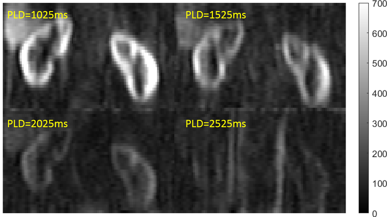
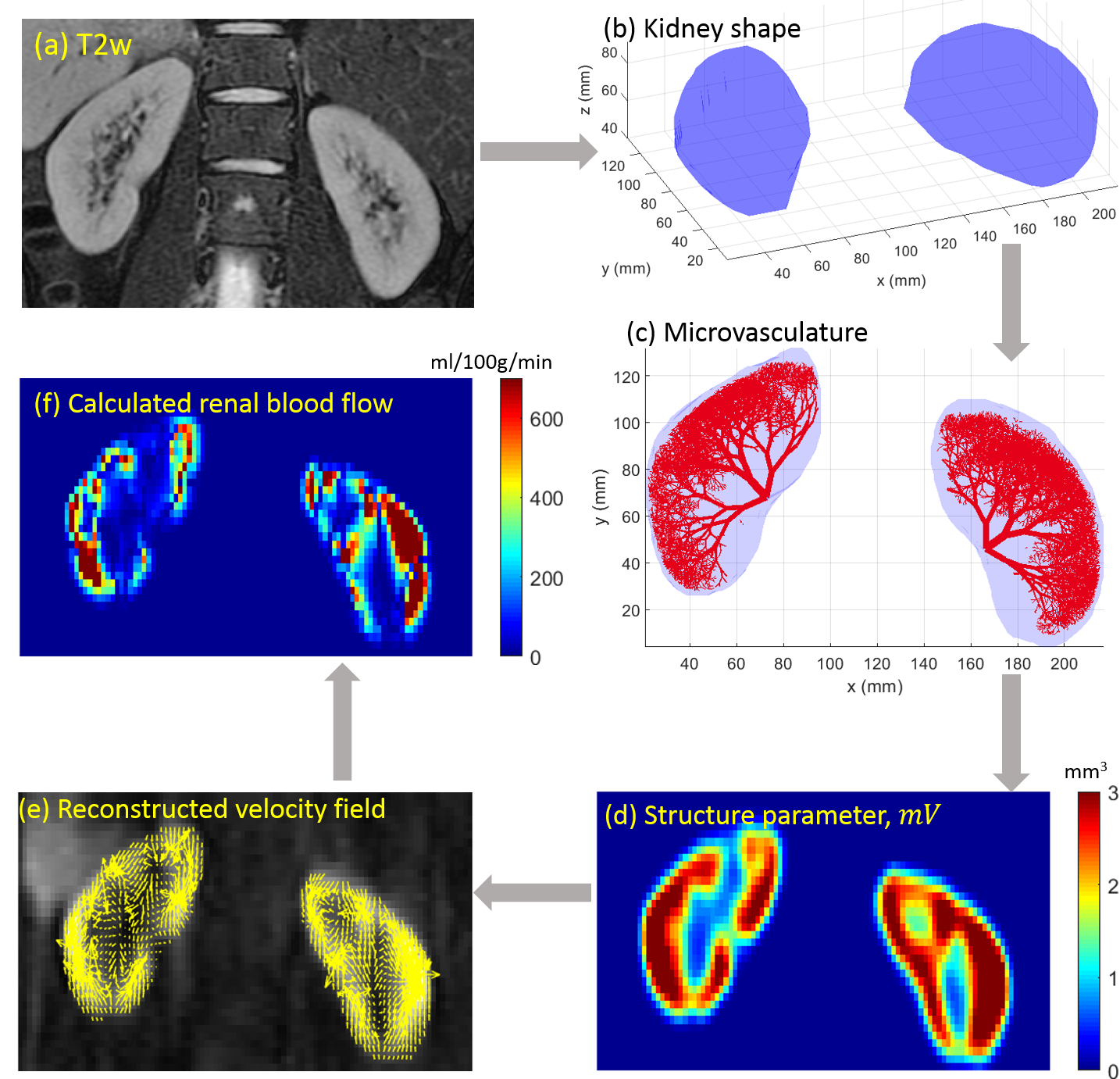
The PMs were calculated from the constructed microvasculature. They were scaled such that the $$$V_m({\boldsymbol\xi})$$$ was approximately equal to the normal renal blood volume of $$$16\%$$$7,8. Using the four post-labeling-delay (PLD=1025ms, 1525ms, 2025ms, 2525ms) ASL data as shown in Fig.1, the QTM is performed and the workflow of QTM is summarized in Fig.2.
Results
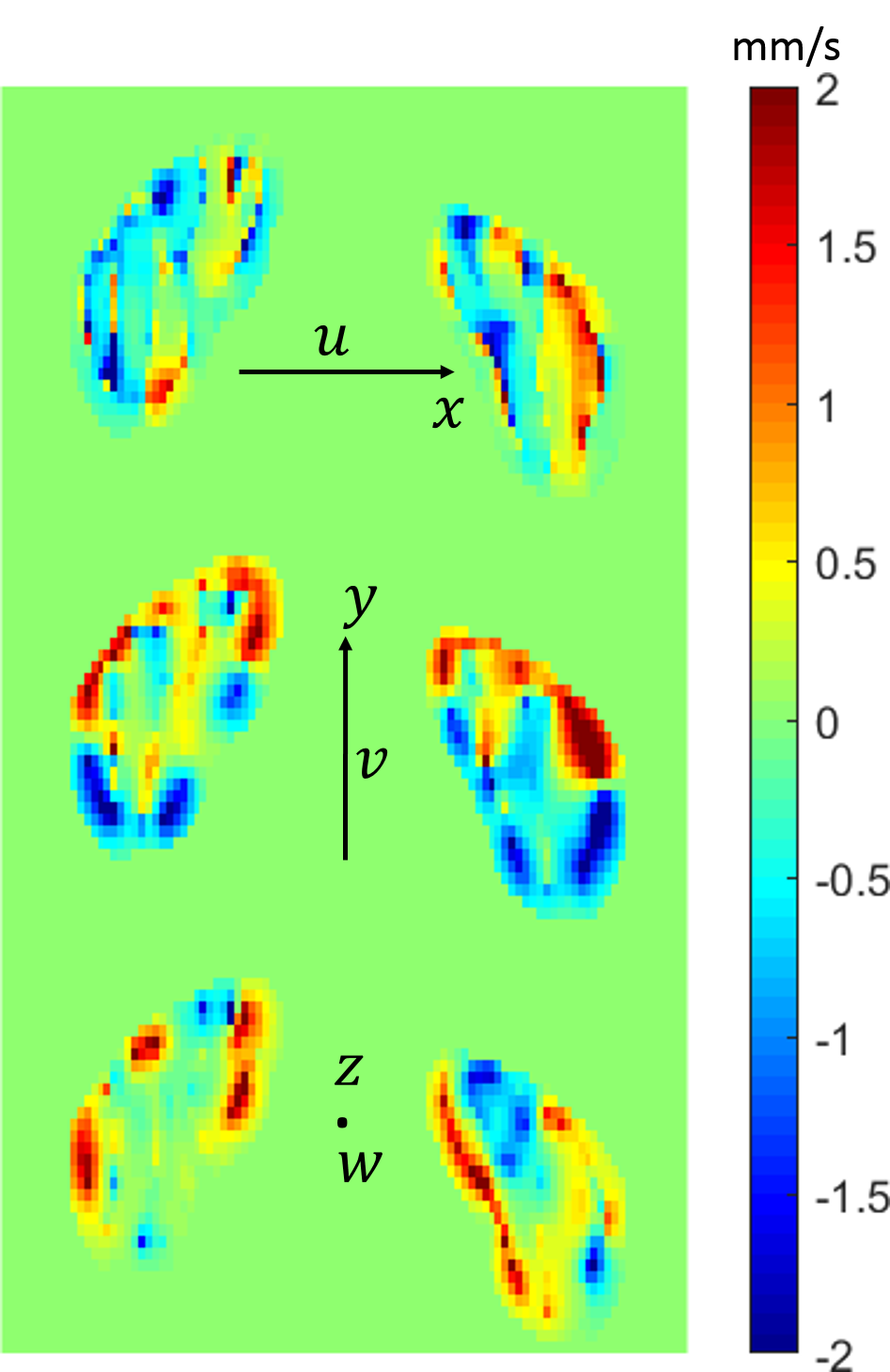
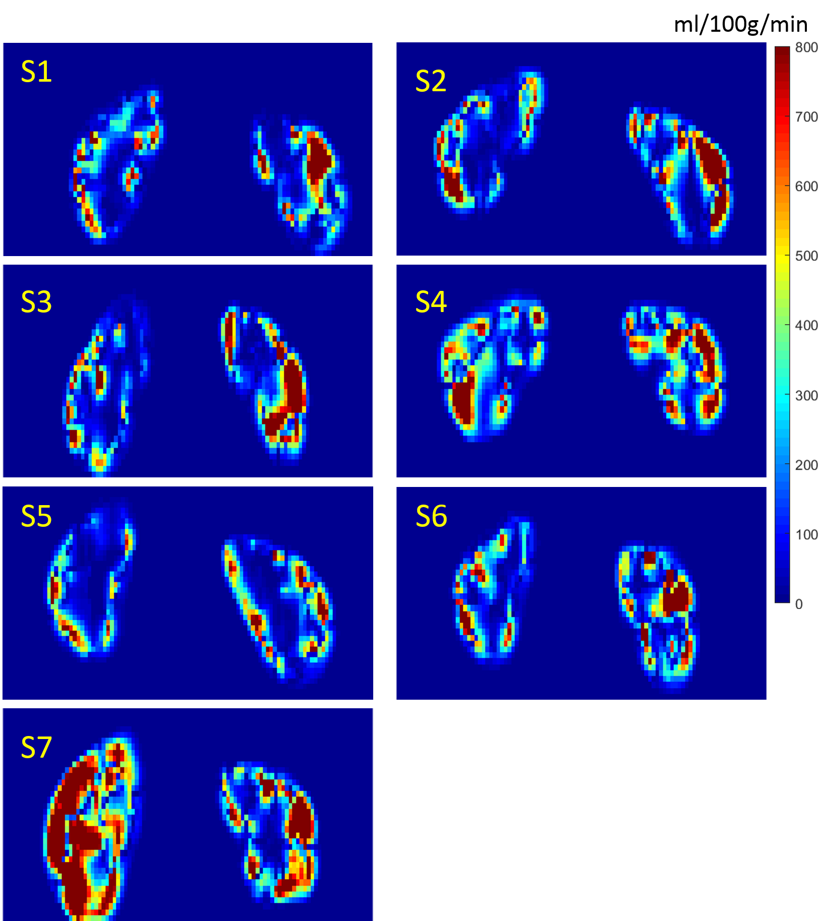
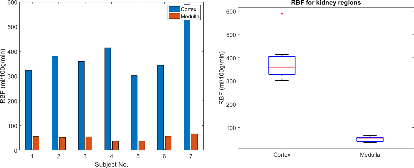
Figure 3 shows the reconstructed blood velocity field for Subject 2. The direction of the velocity can be seen in Figure 2e. Figure 4 shows the RBF quantification in all 7 healthy subjects. Figure 5 shows the obtained RBF values for healthy subjects. Averaged RBF was $$$\,387\pm96\,ml/100g/min$$$ in the cortex compared to $$$51\pm11\,ml/100g/min$$$ in the medulla. These values agree with literature values obtained using conventional ASL post-processing 7,8,9.Discussion
The preliminary data in this work shows the feasibility of QTM to estimate renal blood flow based on a biophysically justified spatio-temporal model of blood flow and an assumed vessel microstructure based on known anatomy and vessel density. In 7 healthy subjects, the flow estimated using the proposed method fell within the range reported in the literature for healthy subjects. A major advantage of the proposed method is that identifying or assuming an AIF is no longer necessary. With an approximate and organ specific microvasculature, QTM can also be applied to other organs like the brain, liver, and breast.
Conclusion
The reconstructed velocity field and blood flow for healthy subjects demonstrate the promise of QTM for assessing blood perfusion without the requirement of a measured or assumed AIF.Acknowledgements
References
1. Kety SS. The Theory and Application of the exchange of inert gas at the lungs and tissues. Pharmacol. Rev. 3(1):1-41, 1951.
2. Calamante F. Arterial Input Function in Perfusion MRI: A Comprehensive Review. Prog. Nucl. Mag. Reson. Spectrosc. 74:1-32, 2013.
3. Spincemaille P, Zhang Q, Nguyen TD, Wang Y. Vector Field Perfusion Imaging. Proc. Intl. Soc. Mag. Recon. Med. 25, 2017.
4. Zhou L, Spincemaille P, Zhang Q, Nguyen TD, Wang Y. Vector Field Perfusion Imaging: A validation Study by using Multiphysics model. Proc. Intl. Soc. Mag. Recon. Med. 26, 2018.
5. Horn BKP, Schunck BG. Determining Optical Flow. Artif. Intl. 17(1-3):185-203, 1981.
6. Nordsletten DA, Blackett S, Bentley MD, Ritman EL, and Smith NP. Structural morphology of renal vasculature. Am J Physiol Heart Circ Physiol 291: H296–H309, 2006.
7. Gillis KA, McComb C, Patel RK, Stevens KK, Schneider MP, Radjenovic A, Morris ST, Roditi GH, Delles C, Mark PB. Non-Contrast Renal Magnetic Resonance Imaging to Assess Perfusion and Corticomedullary Differentiation in Health and Chronic Kidney Disease. Nephron, 133(3):183-192, 2016.
8. Odudu A, Nery F, Harteveld AA, Evans RG, Pendse D, Buchanan CE, Francis ST, Fernández-Seara MA. Arterial spin labeling MRI to measure renal perfusion: a systematic review and statement paper. Nephrol Dial Transplant, 33:15-21, 2018.
9. Nitzsche EU, Choi Y, Killion D, Hoh CK, Hawkins RA, Rosenthal JT, Buxton DB, Huang SC, Phelps ME, Schelbert HR. Quantification and parametric imaging of renal cortical blood flow in vivo based on Patlak graphical analysis. Kidney Intl., 44(5):985-996, 1993.
Figures