0692
Ultra-high temporal resolution on the inversion recovery curve: new insight into T1 relaxometry of the human brain1Institute of Neuroscience and Medicine (INM-4), Research Centre Juelich, Juelich, Germany, 2JARA-BRAIN-Translational Medicine, Research Centre Juelich, Aachen, Germany, 3Institute of Neuroscience and Medicine (INM-11, JARA), Research Centre Juelich, Juelich, Germany, 4Department of Neurology, RWTH Aachen University, Aachen, Germany
Synopsis
Tissue T1 relaxation is considered to be monoexponential. This is, however, an assumption, since it is seldom measured with sufficiently dense sampling of the relaxation curve. We hypothesized that a spatially-resolved investigation of tissue T1 relaxation curve with ultra-high temporal resolution might reveal previously unidentified characteristics of this fundamental NMR parameter. We imaged 10 healthy volunteers using a Look-Locker sequence with 460 time points 17ms apart on the inversion recovery curve. Denoising using PCA and NNLS decomposition of the recovery curves revealed, among others, a moderately short T1 component (4-500ms) in both WM and GM, tentatively assigned to myelin water.
Introduction
NMR relaxation times are known to reflect microscopic tissue properties, albeit in a convoluted way. T2 relaxometry in human white matter reproducibly detects a fast-relaxing component (15ms) attributed to myelin water1 and histologically validated as a myelin marker2. Conventionally, T1 relaxation is considered monoexponential. However, a small number of studies report identification of T1 multicomponent structure3,4 in healthy brain tissue. A methodological difference exists between the investigation of T2 and T1 relaxation curves. Whereas for spin-echo acquisitions of T2 it is feasible, even clinically, to acquire 32 and more echoes per phase-encoding line, it is more time consuming to do so for T1 relaxometry. The reported number of T1 points acquired for investigations of multicomponent relaxation can reach 1285 , but not in conjunction with imaging. Furthermore, the points are often logarithmically-spaced, covering a broad T1 interval (ms-s), leaving relevant T1 regions insufficiently sampled. We hypothesized that a spatially-resolved investigation of the T1 relaxation curve with ultra-high temporal resolution might reveal previously unidentified characteristics of this fundamental NMR parameter.Materials and Methods
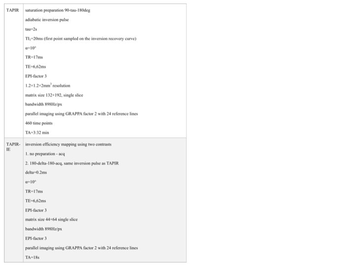
Ten healthy volunteers (5 female, 32.4±0.3yrs) were measured on a 3T MR scanner following prior, written informed consent. Quantitative MRI was performed using a Look-Locker sequence, TAPIR6,7, including mapping of the inversion efficiency. The inversion-recovery curved was sampled in steps of 17ms with 460 time-points within a single-slice TA of ~4 min (Table I). Multi-contrast magnitude and phase data were saved and processed off-line. A ‘noise scan’ was acquired with the same imaging parameters by setting the RF voltage to zero. Analysis of signal characteristics and denoising of magnitude and phase data was performed using principal component (PCA) decomposition of the complex data8, found to be very stable over the 10 volunteers. Only 3-5 components out of 460 contained information relevant to signal decay. For each volunteer, the number of signal-containing components was assessed visually and also inferred from random matrix theory analysis of the distribution of eigenvalues9. Furthermore, a comparison of eigenvalue spectra from signal and noise regions and from acquisitions of noise only was performed and characteristics of noise spectra identified. Noise-only components were discarded. Monoexponentially fitting the TAPIR signal7 delivered maps of the longitudinal relaxation time T1, signal intensity at TI=0 and flip angle. The effect of data denoising on fit parameters was investigated. NNLS analysis using 200 logarithmically spaced T1 values between 50ms and 6s and Tikhonov regularisation was performed on the original, noisy data, and after denoising. Masks for different tissue types were defined using simultaneously acquired MPRAGE and SPM-based segmentation. The components identified in the T1 spectra are reported per tissue class and their distribution visualised as maps of component fractions.
Results
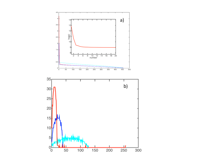
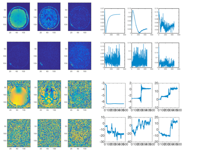
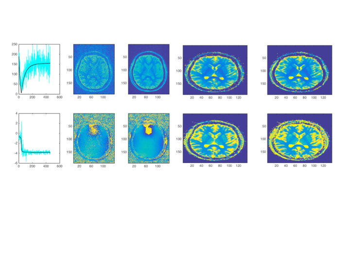
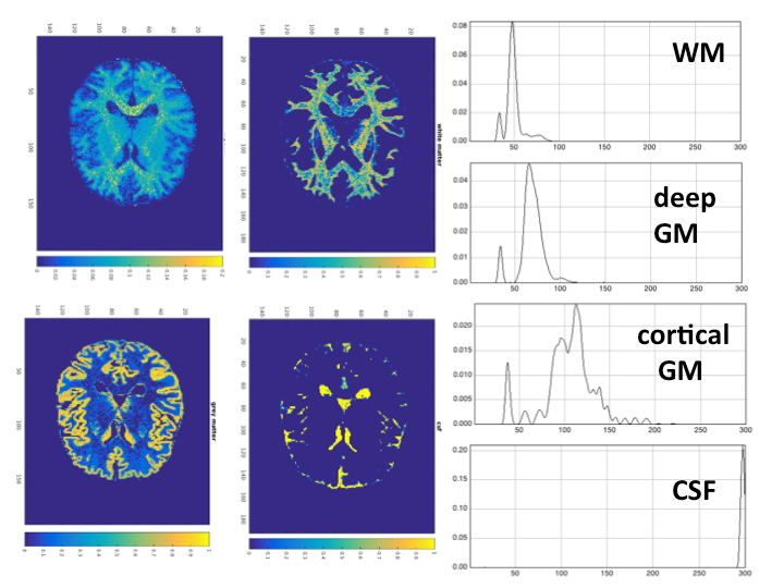
The salient features of the PCA decomposition are illustrated in Figs. 1-2. Fig.1 describes the behaviour of eigenvalues obtained from analysing the signal from the brain region and the corresponding characteristics of the noise spectrum; the latter is obtained either from regions void of signal, or from the noise acquisition. The first 6 principal components are shown in Fig.2a and their temporal characteristics in Fig.2b, separately for magnitude and phase. The effects of denoising are characterised in Fig.3 for the signal obtained from a single GM voxel and the images at time point 19 (TI=343ms) (Fig 3a), and the T1 and M0 maps obtained by monoexponential fitting of the data (Fig.3b). Fig.4 shows the results of NNLS analysis of the denoised data, with Tikhonov regularisation (chi2<1.025*chi2_orig), in spectra and image form.Discussion and Conclusion
In practically all WM and GM voxels a short T1 component was identified, with T1~400ms (WM) and ~500ms(GM), also when using original low-SNR data. In the absence of regularisation, an additional, even shorter component might be present; however, only the longer short component survives regularisation. The presence of a transient, MT-induced, short relaxation component in Look-Locker acquisitions is well known10. However, biexponential decay due to MT only affects the first 60-100ms on the inversion curve10, giving a T1 component with an order-of-magnitude shorter time constant than the ~500ms found here. In conclusion, a distinct, moderately short T1 component is robustly identified in vivo, arguably for the first time. The maps reflecting its spatial distribution show unprecedented SNR and detail for multicomponent relaxometry, even when analysis is performed on the original (SNR=10) data. While in WM a single additional peak was identified in most cases, GM shows a more complicated T1 spectrum. The precise nature of these components requires further investigation11.Acknowledgements
No acknowledgement found.References
[1] A. MacKay, K. Whittall, J. Adler, D. Li, D. Paty, D. Graeb. In vivo visualization of myelin water in brain by magnetic resonance. Magn. Reson. Med., 31 (6) (1994), pp. 673-677
[2] C. Laule, P. Kozlowski, E. Leung, D.K. Li, A.L. Mackay, G.R. Moore. Myelin water imaging of multiple sclerosis at 7 T: correlations with histopathology. Neuroimage, 40 (2008), pp. 1575-1580
[3] C. Labadie, J.H. Lee, W.D. Rooney, S. Jarchow, M. Aubert-Frecon, C.S. Springer Jr., H.E. Moller. Myelin water mapping by spatially regularized longitudinal relaxographic imaging at high magnetic fields. Magn. Reson. Med., 71 (1) (2014), pp. 375-387
[4] R. Barta, S. Kalantari, C. Laule, I.M. Vavasour, A.L. MacKay, C.A. Michal. Modeling T1 and T2 relaxation in bovine white matter. Journal of Magnetic Resonance 259, 2015, p56-67, https://doi.org/10.1016/j.jmr.2015.08.001.
[5] Mark D. Does, Christian Beaulieu, Peter S. Allen, Richard E. Snyder. Multi-component T1 relaxation and magnetisation transfer in peripheral nerve. Magnetic Resonance Imaging 16, 1998, p 1033-1041
[6] Shah, N. J., Neeb, H., Zaitsev, M., Steinhoff, S., Kircheis, G., Amunts, K., . . . Zilles, K. (2003). Quantitative T1 mapping of hepatic encephalopathy using magnetic resonance imaging. Hepatology, 38(5), 1219-1226. doi:10.1053/jhep.2003.50477
[7] Zaitsev, M., Steinhoff, S., & Shah, N. J. (2003). Error reduction and parameter optimization of the TAPIR method for fast T1 mapping. Magn Reson Med, 49(6), 1121-1132. doi:10.1002/mrm.10478
[8] I.T. Jolliffe. Principal Component Analysis (Springer Series in Statistics) 2nd Edition ISBN-13: 978-0387954424
[9] Veraart, J., Novikov, D. S., Christiaens, D., Ades-Aron, B., Sijbers, J., & Fieremans, E. (2016). Denoising of diffusion MRI using random matrix theory. NeuroImage, 142, 394-406. doi:10.1016/j.neuroimage.2016.08.016
[10] Li, K., Li, H., Zhang, X. Y., Stokes, A. M., Jiang, X., Kang, H., . . . Xu, J. (2016). Influence of water compartmentation and heterogeneous relaxation on quantitative magnetization transfer imaging in rodent brain tumors. Magn Reson Med, 76(2), 635-644. doi:10.1002/mrm.25893
[11] A.M. Oros et al, submitted to present ISMRM
Figures