0681

Inhomogeneous Neural Network Inversion (NNI_inh) for stiffness estimation in Magnetic Resonance Elastography

Jonathan M Scott¹, Arvin Arani², Armando Manduca³, John Huston III², Richard L Ehman², and Murphy C Matthew²

¹Medical Scientist Training Program, Mayo Clinic, Rochester, MN, United States, ²Radiology, Mayo Clinic, Rochester, MN, United States, ³Biomedical Engineering and Physiology, Mayo Clinic, Rochester, MN, United States

Synopsis

Stiffness estimates in small focal lesions by magnetic resonance elastography are often inaccurate. One factor contributing to these errors is the assumption of local material homogeneity made by most inversion algorithms. Here we describe an artificial neural network based inversion technique that accounts for material inhomogeneity (NNI_inh) and evaluate it in simulation, phantom, and in-vivo experiments. NNI_inh provides higher contrast-to-noise ratio for inclusions and may provide clearer delineation of inclusion boundaries when compared to two inversion algorithms that assume local material homogeneity. Preliminary clinical results in a case of hepatocellular carcinoma are also shown.

Introduction

Magnetic Resonance Elastography (MRE) is a phase contrast MRI technique for noninvasive measurement of tissue mechanical properties¹. In focal disease, stiffness has been shown to differentiate benign from malignant tumors in the liver², pancreas³, and brain⁴, as well as characterize brain tumor mechanical properties for preoperative planning^5,6. While these applications are promising, small (<2cm) focal lesions are often unable to be evaluated due to limited spatial resolution^2,3,5. Inversion algorithms that estimate mechanical properties from acquired wave displacement fields are one of the factors limiting the spatial resolution of stiffness maps. Most of these algorithms assume homogeneous stiffness within a patch of an image^7,8, and those that do not require acquisition of data at multiple frequencies⁹ or long computation times¹⁰. In this study we describe an inversion technique that allows for local inhomogeneity by training an artificial neural network (ANN) on a viscoelastic simulation of wave propagation in a medium with inhomogenenous stiffness. We present initial results for the new inversion (NNI_inh) and compare it with a previously reported homogeneously trained neural network inversion (NNI_hom)⁷, direct inversion (DI)¹¹, and multiple model direct inversion (MMDI)¹² in simulation, phantom, and in-vivo studies.

Methods

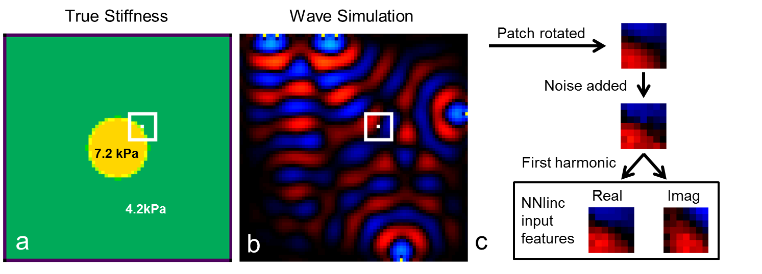
Training Data Generation: A coupled harmonic oscillators (CHO) simulation adapted from Braun et al.^13,14 was used to generate 104000 simulated datasets. Each simulation had the geometry described in Figure 1. All simulation variables (inclusion stiffness, background stiffness, sphere diameter, and number of wave sources) were randomly selected from a uniform distribution for each simulation. 100 7x7x7 pixel patches were taken from near the boundary of the inclusion from each simulated dataset. ANN input features were the real and imaginary components of the temporal first harmonic of each patch. Training data for NNI_hom was generated as described in Murphy et al.⁷. An analogous process with 100Hz wave sources in 2D was used to generate training data for a 2D version of the algorithms.

Neural Network Inversion: For both NNI_inh and NNI_hom in 3D, a fully-connected, feed-forward ANN composed of 3 hidden layers each containing 1000 units with rectified linear unit transfer functions was trained on 10 million examples using RMSProp¹⁵ with a batch size of 1000 and a mean squared error (MSE) loss function. Three decreasing learning rates were used, and training at each learning rate was stopped after three consecutive iterations where the MSE did not improve in the validation set (200,000 held out examples). The output of the network is a stiffness estimate (kPa) for the center voxel of the patch. The 2D versions of NNI_hom and NNI_inh were trained with a previously described ANN architecture⁷. 2D inversions are used only in the four-cylinder phantom experiment; all other experiments use 3D inversions.

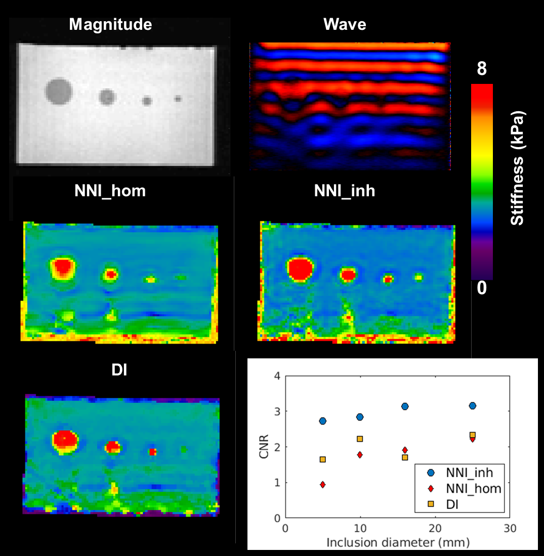
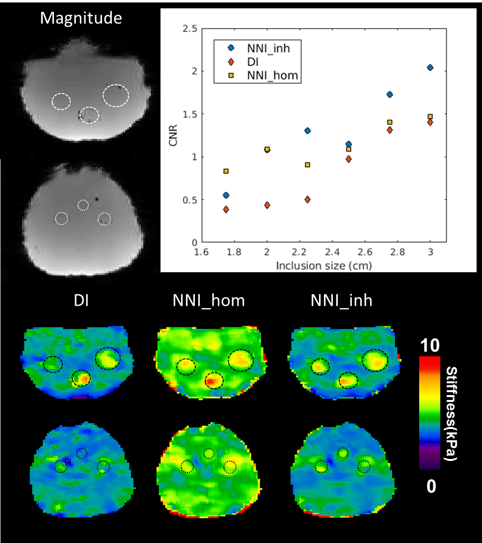
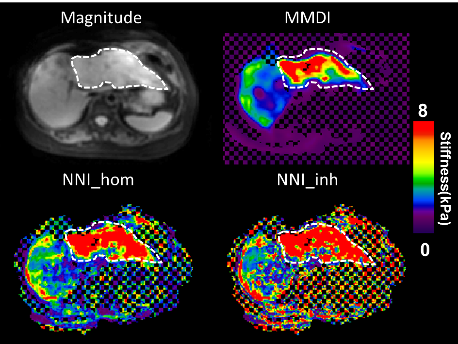
Image Acquisition: 2D MRE at 100Hz was performed on an agar and bovine gelatin phantom with four stiff cylindrical inclusions in a soft background as previously described¹⁶. 3D MRE was performed on a polyvinyl chloride brain phantom with embedded spherical inclusions on a compact 3T system using a modified 3D GRE pulse sequence at 60Hz with 2mm isotropic resolution¹⁷. The liver example shown was acquired on a 1.5T MR scanner (GE Medical System, Milwaukee, WI) using a previously described acquisition protocol at 60Hz^18,19.

Results

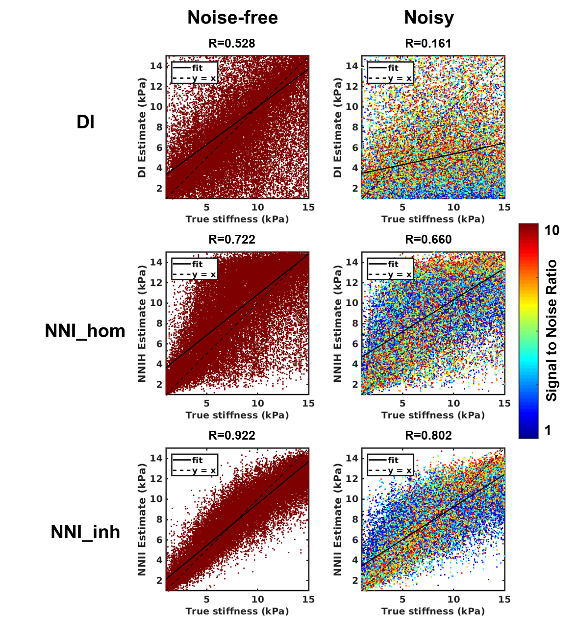
Performance of NNI_inh, NNI_hom, and DI (with 3x3x3 quartic smoothing) on the NNI_inh test set is shown in Figure 2. NNI_inh estimates show higher correlation with the true stiffness than those of NNI_hom and DI. In the four-cylinder phantom (Figure 3), NNI_inh provided a higher contrast to noise ratio (CNR) and sharper delineation of the inclusions when compared to NNI_hom and DI. In the brain phantom (Figure 4), NNI_inh provides similar or higher CNR than DI and NNI_hom for the five largest inclusions. All three inversions struggle to detect the smallest lesion, though NNI_hom provides the highest CNR (0.83). In the liver tumor case (Figure 5), 3D NNI_hom and NNI_inh better capture the full extent of the tumor than MMDI, while NNI_inh provides slightly less blurring at the tumor boundary.

Discussion and Conclusions

By incorporating inhomogeneous training data, NNI_inh was able to more clearly delineate the margins of the liver tumor and inclusion boundaries in the four cylinder phantom than inversions assuming material homogeneity. In the brain phantom, the 3D NNI_inh inversion provided improved CNR for most inclusions, but failed to detect the smallest inclusion or provide clearer delineation of inclusion boundaries. While needing further tuning in 3D, this approach may allow improved delineation of focal lesion margins and detection of smaller focal lesions than possible with approaches assuming material homogeneity.

Acknowledgements

This research was supported by the National Institute of Biomedical Imaging and Bioengineering (NIBIB) of the National Institutes of Health (NIH) under award number R37-EB001981.

References

1. Muthupillai, R. et al. Magnetic resonance elastography by direct visualization of propagating acoustic strain waves. Science 269, 1854–1857 (1995).

2. Venkatesh, S. K. et al. MR elastography of liver tumors: preliminary results. AJR Am J Roentgenol 190, 1534–1540 (2008).

3. Shi, Y. et al. Differentiation of benign and malignant solid pancreatic masses using magnetic resonance elastography with spin-echo echo planar imaging and three-dimensional inversion reconstruction: a prospective study. Eur Radiol 28, 936–945 (2018).

4. Pepin, K. M. et al. Magnetic resonance elastography analysis of glioma stiffness and IDH1 mutation status. AJNR Am J Neuroradiol 39, 31–36 (2018).

5. Hughes, J. D. et al. Higher-Resolution Magnetic Resonance Elastography in Meningiomas to Determine Intratumoral Consistency. Neurosurgery 77, 653–659 (2015).

6. Murphy, M. C. et al. Preoperative assessment of meningioma stiffness using magnetic resonance elastography. J. Neurosurg. 118, 643–648 (2013).

7. Murphy, M. C. et al. Artificial neural networks for stiffness estimation in magnetic resonance elastography. Magnetic Resonance in Medicine 80, 351–360

8. Manduca, A. et al. Magnetic resonance elastography: Non-invasive mapping of tissue elasticity. Medical Image Analysis 5, 237–254 (2001).

9. Barnhill, E. et al. Heterogeneous Multifrequency Direct Inversion (HMDI) for magnetic resonance elastography with application to a clinical brain exam. Medical Image Analysis 46, 180–188 (2018).

10. Houten, E. E. W. V., Miga, M. I., Weaver, J. B., Kennedy, F. E. & Paulsen, K. D. Three-dimensional subzone-based reconstruction algorithm for MR elastography. Magnetic Resonance in Medicine 45, 827–837

11. Oliphant, T. E., Manduca, A., Ehman, R. L. & Greenleaf, J. F. Complex-valued stiffness reconstruction for magnetic resonance elastography by algebraic inversion of the differential equation. Magn Reson Med 45, 299–310 (2001).

12. Silva, A. M. et al. Magnetic resonance elastography: evaluation of new inversion algorithm and quantitative analysis method. Abdom Imaging 40, 810–817 (2015).

13. Sack, I., Bernarding, J. & Braun, J. Analysis of wave patterns in MR elastography of skeletal muscle using coupled harmonic oscillator simulations. Magn Reson Imaging 20, 95–104 (2002).

14. Braun, J., Buntkowsky, G., Bernarding, J., Tolxdorff, T. & Sack, I. Simulation and analysis of magnetic resonance elastography wave images using coupled harmonic oscillators and Gaussian local frequency estimation. Magnetic Resonance Imaging 19, 703–713 (2001).

15. Hinton, G. Neural Networks for Machine Learning - Lecture 6a - Overview of mini-batch gradient descent. (2012).

16. Manduca, A., Lake, D. S., Kruse, S. A. & Ehman, R. L. Spatio-temporal directional filtering for improved inversion of MR elastography images. Medical Image Analysis 7, 465–473 (2003).

17. Scott, J. M. et al. Estimating Inclusion Stiffness with Artificial Neural Networks in Magnetic Resonance Elastography. in International Society for Magnetic Resonance in Medicine 3496, (2018).

18. Dzyubak, B. et al. Automated Liver Stiffness Measurements with Magnetic Resonance Elastography. J Magn Reson Imaging 38, 371–379 (2013).

19. Yin, M. et al. Assessment of hepatic fibrosis with magnetic resonance elastography. Clin. Gastroenterol. Hepatol. 5, 1207-1213.e2 (2007).

Figures

Figure 1. Summary of training data generation. (a) An underlying stiffness map is generated at 2-mm isotropic resolution by placing a spherical inclusion (5-25 pixel diameter, 1-15kPa stiffness) inside of a homogenous background (41x41x41 pixels, 1-15kPa). (b) 60Hz point-source harmonic force generators are randomly placed at the simulation boundary. (c) 100 7x7x7 pixel patches (white square in (a) and (b)) are taken from near the boundary of the inclusion in each simulation. Each patch is rotated and has Gaussian noise added such that the SNR within each patch varies from 1-10.

Figure 2. Direct inversion (DI, top row), Homogeneous Neural Network Inversion (NNI_hom, middle row), and Inhomogeneous Neural Network Inversion (NNI_inh, bottom row) results in a test set of 200,000 patches within one pixel of the boundary of the inclusion. Results for noise-free patches (first column) and noisy patches (SNR 1-10, second column) are shown. Both NNI_hom and NNI_inh were trained on noisy data with SNR ranging from 1 to 10.

Figure 3. Inversion results in the four cylinder phantom. 2D versions of NNI_inh and NNI_hom for this experiment were trained over the stiffness range of 1-10kPa and SNR range of 1-20 at a frequency of 100Hz to match characteristics of the acquired wave data. Inclusion diameters are (left to right): 25 mm, 16mm, 10mm, and 5mm. Background stiffness is ~2.9kPa and inclusion stiffness is ~6.4 kPa, as estimated by MRE in separately poured homogeneous phantoms.

Figure 4. Inversion results in the brain phantom with inclusions. Inclusion diameters are (left to right, top to bottom): 2.5cm, 2.75cm, 3cm, 2.25cm, 2.0cm, 1.75cm. Background stiffness is ~3.5kPa and inclusion stiffness is ~7.0kPa as estimated by mechanical testing. Note that slices were chosen such that all six inclusions can be displayed in two slices, and the slice may not pass through the center of one or more of the inclusions.

Figure 5. Inversion results in a case of biopsy proven hepatocellular carcinoma in the left lobe of the liver. MMDI is designed to give stable estimates over large regions, and as a result blurs the margins of the tumor while NNI_hom and NNI_inh both better capture its full extent. The checkerboard pattern covers regions of the inversion images with MMDI confidence under 95%.

Proc. Intl. Soc. Mag. Reson. Med. 27 (2019)

0681