0680
Variational vs Adversarial Autoencoders for Visualization and Interpretation of Deep Learning Features of Brain Aging1Biomedical Engineering, Hotchkiss Brain Institute, University of Calgary, Calgary, AB, Canada, 2Seaman Family MR Research Centre, Foothills Medical Centre, Calgary, AB, Canada, 3Radiology and Clinical Neurosciences, Hotchkiss Brain Institute, University of Calgary, Calgary, AB, Canada, 4Calgary Image Processing and Analysis Centre, Foothills Medical Centre, Calgary, AB, Canada
Synopsis
Deep learning models are state-of-the-art for numerous medical imaging prediction tasks. Exact understanding of learned prediction features is hard, slowing down their clinical application. New methods for interpreting such models are needed to enable clinical translation. Autoencoders are models that allow visualization of learned features, however they can lack detail in their visualizations and thus, cannot provide guidance on features that hinders their use. We propose a method for understanding relevant learned features by visualizing them in detailed images. We show that a model trained to predict age based on brain MR data learns known features of the aging brain.
Introduction
Deep learning (DL), an emerging field of artificial intelligence, has allowed unprecedented performance in numerous medical imaging challenges such as segmentation and classification by automatically extracting relevant features within large amounts of data. An underlying issue of such approaches is that their learned features are not easily interpretable for experts due to their high complexity, which deteriorates our ability to explain DL predictions, furthermore imposing a challenge for practical applicability of such techniques.1 Autoencoders are deep learning models that map image information into compressed latent representation (LR) features via an encoder, then tries to reconstruct the original image from the LR via a decoder. The LR is forced to encode the most important features of the images, so that reconstruction is possible.2 In a previous work, ventricle size changes were observed when reconstructing images by decoding LR features using an adversarial variational autoencoder modified to predict age based on brain MR images.3 However, inherent constraints of the model minimized reconstruction capabilities, forcing it to reconstruct filtered images, subsequently limiting further interpretation of results. In this work, we propose a DL model capable of generating sharper, more realistic reconstructions, allowing for easier interpretability of learned LR features. We apply the model to predict age based on brain MR images. We show that the model learns internal representations of changes in ventricle size and sulci shapes to predict age more accurately.Methodology
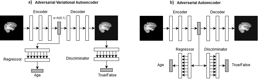
The proposed model architecture is shown in Figure 1b. The model is a convolutional adversarial autoencoder4 modified with two additions: a regressor, used to predict age; and a discriminator model, used to regularize the LR. Previously, a discriminator was used to train the autoencoder to generate realistic output reconstructions, while an artificial constraint was applied for the LR to be normally distributed. Because details of the high frequencies are embedded into the LR, if the LR doesn’t represent the image optimally, image details wouldn’t be able to be reconstructed. This forced the model to output realistic but blurry reconstructions. The newly proposed discriminator, however, is used not to constrain, but to regularize the LR to approximate a normal distribution, without looking at the output reconstruction. With adversarial autoencoders, the discriminator assures that the LR is realistic as compared to a prior normal distribution but doesn’t interfere directly with the reconstruction process of the decoder. Hence, the discriminator and the regressor force the LR to encode age information and detailed LR features of the images, leading to simultaneously realistic and detailed reconstructions. We trained our models on a subset of the Alzheimer’s Disease Neuroimaging Initiative (ADNI) dataset with T1-weighted sagittal images of ~2,200 cognitively normative subjects aged 56 to 90. The images were skull stripped, co-registered, intensity normalized, and separated into training and testing sets (70%:30% split). We use integrated gradients5 technique to visualize attributes of the image relevant for predictions. The independent components of the LR were obtained via independent component analysis.Results
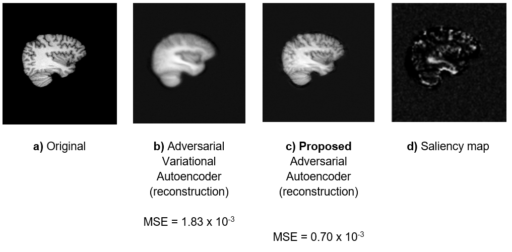
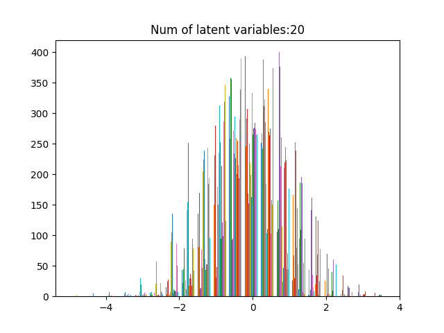
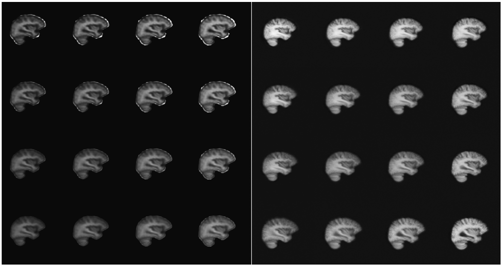
The proposed model obtained a mean absolute error (MAE) of age prediction on the test dataset of 1.6±0.8 years, a 48% reduction of previous algorithm (3.1±1.3 years). As shown in Figure 2, proposed model achieved a 61% lower mean squared error (MSE), resulting in more detailed images. Figure 2d highlights features that were most relevant for the age prediction; highlighted features include the ventricles and sulci. Figure 3 shows the distribution of latent features. Figure 4 shows sample reconstructions from two decoded independent component axes.Discussion
The improved accuracy in age prediction can be explained by a better LR of the image features, also allowing the proposed model to reconstruct the original images with higher details compared to previously proposed algorithm. This allows for further investigation and interpretability of results obtained by deep learning models. For example, by using saliency maps (Figure 2d), we show that the image regions which influence the age prediction of the model are ventricle size and sulci spacings, known features of the aging brain. In Figure 4, it is possible to visualize the LR axis where ventricle size was encoded.Conclusion
As deep learning is being used to solve more critical problems in medicine, understanding these models is a priority in order to avoid unexpected failures when put into clinical practice. In this work, we approached the problem of model interpretability by proposing a model that can look inside learned features allowing us to visualize what is being learnt. In the future, we aim to use our proposed model to understand the disease progression between early and late cognitively impaired brains by visualizing their feature representations.Acknowledgements
No acknowledgement found.References
1. Zhang Q, Zhu S. Visual interpretability for deep learning: A survey. CoRR, vol. abs/1802.00614, 2018. Available: http://arxiv.org/abs/1802.00614
2. Goodfellow I, Bengio Y, Courville A. Deep Learning. MIT Press, 2016, Available: http://www.deeplearningbook.org
3. Souto Maior Neto LA, Bento M, Gobbi D, Salluzzi M, Frayne R. Adversarial variational autoencoder for visualizing and interpreting deep features of brain aging. ISMRM Machine Learning Workshop 2018. [abstract]. Available: https://cds.ismrm.org/protected/Machine18II/program/abstracts/orals/SoutoMaior.pdf
4. Makhzani A, Shlens J, Jaitly N, Goodfellow IJ. Adversarial autoencoders. CoRR. vol. abs/1511.05644, 2015. Available: http://arxiv.org/abs/1511.05644
5. Sundararajan M, Taly A, Yan Q. Axiomatic attribution for deep networks. CoRR, vol. abs/1703.01365, 2017. Available: http://arxiv.org/abs/1703.01365
Figures