0678

Visualizing and understanding deep learning features for MRI motion artifact detection

Irene Heleonora Sêda Pinto Fantini¹, Letícia Rittner¹, Clarissa Lin Yasuda², and Roberto Alencar Lotufo¹

¹School of Electrical and Computer Engineering, UNICAMP, Campinas, Brazil, ²Faculty of Medical Sciences, UNICAMP, Campinas, Brazil

Synopsis

The high performance reported by Deep Convolutional Neural Networks (CNNs) on image classification, detection and segmentation are contributing to its usage increase, including the CNNs applied to Medical Image. To automatically detect motion artifacts on MRI we fine-tuned four different CNNs. Visualizing the features extracted by the CNN is crucial to understand the reported result from each architecture. Using a gradient-based visualization method, we noticed that all architectures have salient points on Cerebrospinal Fluid (CSF) and background. Furthermore, the architectures that reported better results also extract information from white-matter, confirming that this anatomical structure has essential information regarding the task.

Introduction

Deep Convolutional Neural Networks (CNNs) are evolving and reporting high performance on image classification, detection, and segmentation. The method does not require prior image feature extraction, a crucial phase when implementing classical machine learning methods. Performing several convolutions, the CNN learns the relevant features from the dataset to solve the specific problem^1,2. Nowadays several consortia3,4 are creating huge datasets to aid clinical research, demanding a robust, automatic tool to support on quality screening, such as detecting and correcting motion artifacts on Magnetic Resonance Image (MRI)^5,6,7. When working on medical images the understanding of the features extracted by the CNN is essential to analyze the results and make a comparison between methods. This work aims to visualize the saliency map used by the CNN when detecting if the MRI has motion artifacts or not.

Methods

We fine-tuned a modified version of four CNN architectures, Xception⁸, Inception⁹, ResNet¹⁰, and Inception-ResNet¹¹ to detect motion artifacts on MRI⁷. T1-weighted volumetric were acquired in the sagittal plane (thickness = 1 mm, flip angle = 8 degrees, TR = 7.1 msec, TE = 3.2 msec, matrix 240x240x180, isotropic voxels of 1 mm) from healthy volunteers, on a 3T Phillips Achieva scanner. An expert annotated the dataset as a two classes problem, motion-free or motion-corrupted image, resulting on 68 acquisitions: 34 corrupted by motion (25 females, 9 males, age varying from 21 to 61) and 34 motion-free acquisition (balanced by gender and age, varying from 21 to 59). Training was performed on the three axes separately (axial, coronal and sagittal) using 48 volumes and tested on 20 volumes, using 3-fold cross-validation. While the training step utilized image patches, testing was performed on the whole image (both, image and patches, 2D), discarding only the neck area. Patches extraction considered the image inside a bounding box containing the brain structure, with no segmentation, also containing skull and background. A gradient-based visualization method¹² was applied to investigate which characteristics influenced the CNNs results, resulting in a saliency map for each CNN model. This map was obtained calculating the gradients, by backpropagation, from the input images. The CNNs input images have three channels and, since the MRI is grayscale, the same image is used on every channel. The final gradient map considered the maximum value from the three input channels.

Results and Discussion

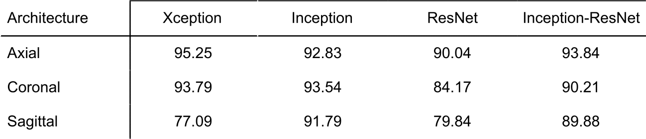
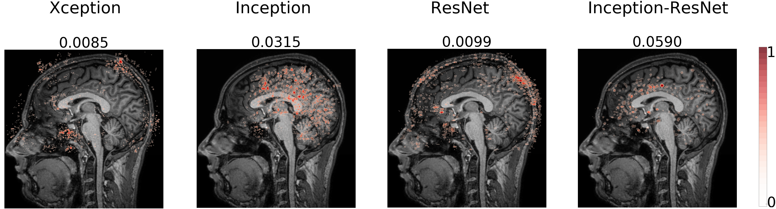
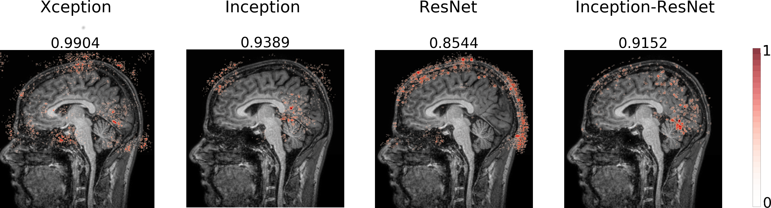
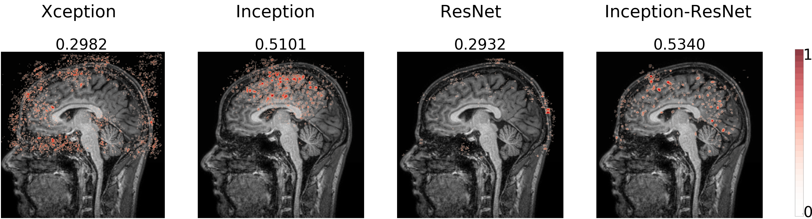
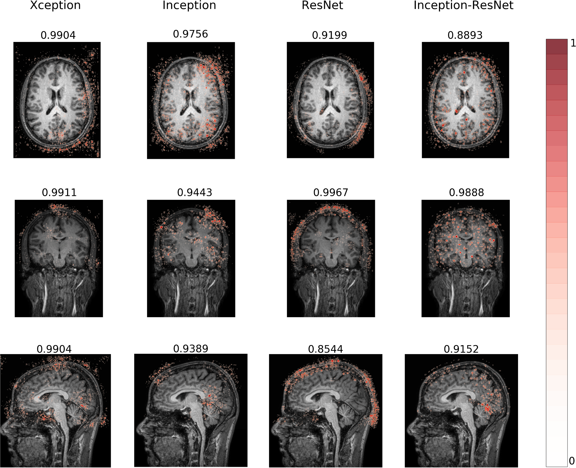
The models are trained to detect the motion artifact in the input image resulting in a probability P ∈ [0, 1] of motion artifact presence. A threshold of 0.5 was used to classify the image and calculate the accuracy. The CNNs trained using the sagittal plane presented the lowest accuracies and the highest variance when compared to the ones trained using the axial and the coronal planes, for every architecture (Table 1). The sagittal plane has some distinct characteristics such as asymmetry, multiple anatomical structures on the same slice and the interhemispheric fissure influence on the mid-sagittal slice. Investigating the reason why the sagittal plane presented such different performance we decided to visualize the CNNs saliency map. Examples of saliency maps from sagittal slice correctly classified as motion-free (Figure 1) and as motion-corrupted (Figure 2) are presented. We noticed salient points from input image located on Cerebrospinal Fluid (CSF) on all architectures. Additionally, Inception and Inception-ResNet architectures extract information from white-matter and interestingly, achieves the highest accuracy on the classification study. One example of unsuccessful classification for the motion-corrupted image (Figure 3) shows false negative result from Xception, which extracts information from several points of the input image, and ResNet, which extracts only a few points located near to the skull. When comparing saliency maps for axial and coronal planes with the sagittal one (Figure 4) we observe that the CNNs have the same behavior. The ResNet architecture extracts information only from the CSF and background, mostly near to the skull area, and presents a considerably lower performance than the Xception, Inception, and Inception-Resnet, suggesting the learning of weak features. Interestingly, Xception, which have a good performance when trained on axial and coronal planes, reports few points and most of them located on the background, confirming the contribution of background for the task¹³.

Conclusions

We presented the visualization of saliency maps from MR Image when a trained CNN automatically detects motion artifacts on it. The MR Image saliency map reveals that architectures which had better performance on detecting motion artifacts have considered information not only from CSF but also from the white-matter suggesting that combining information from several anatomic structures is valuable to the task.

Acknowledgements

This work was supported by the Coordination for the Improvement of Higher Education Personnel (CAPES - scholarship process 1545649/2015-08), the São Paulo Research Foundation (FAPESP - process CEPID 2013/07559-3) and the Brazilian National Council for Scientific and Technological Development (CNPq – process 308311/2016-7).

References

1 Litjens G, Kooi T, Bejnordi , et al. A survey on deep learning in medical image analysis. Medical Image Analysis, 42(December 2012):60–88, 2017.

2 Shen D, Wu G, and Suk H. Deep Learning in Medical Image Analysis. Annual Review of Biomedical Engineering, 19(1):221–248, 6 2017

3 Ollier W, Sprosen T, Peakman T (2005) UK Biobank: from concept to reality. Pharmacogenomics 6(6):639–646

4 Bamberg F, Kauczor HU, Weckbach S, et al. (2015) Whole-body MR imaging in the German National Cohort: rationale, design, and technical background. Radiology 277(1):206–220

5 Iglesias J, Lerma-Usabiaga G, Garcia-Peraza-Herrera L, et al. Retrospective head motion estimation in structural brain MRI with 3D CNNs. Lecture Notes in Computer Science (including subseries Lecture Notes in Artificial Intelligence and Lecture Notes in Bioinformatics. 2017;10434 LNCS:1-8

6 Kustner T, Liebgott A, Mauch L et al. Automated reference-free detection of motion artifacts in magnetic resonance images. Magnetic Resonance Materials in Physics, Biology and Medicine.2018;31(2): 243-256

7 Fantini I, Rittner L, Yasuda C, et al. International Workshop on Pattern Recognition in Neuroimaging (PRNI), Singapore, 2018;

8 Chollet F. Xception: Deep Learning with Depthwise Separable Convolutions. IEEE Conference on Computer Vision and Pattern Recognition (CVPR); 1800-1807,

9 Szegedy C, Vanhoucke V, Ioffe S, et al. Rethinking the inception architecture for computer vision. IEEE Conference on Computer Vision and Pattern Recognition (CVPR), Las Vegas, NV, USA, 2016; 2818-2826

10 He K, Zhang X, Ren S, et al. Deep Residual Learning for Image Recognition. IEEE Conference on Computer Vision and Pattern Recognition (CVPR), Las Vegas, NV, USA, 2016; 770-778

11 Szegedy C, Ioffe S, Vanhoucke V, et al. Inception-v4, inception-resnet and the impact of residual connections on learning. Proceedings of the Thirty-First AAAI Conference on Artificial Intelligence, San Francisco, California, USA, 2017;4278–4284

12 Simonyan K, Vevaldi A, Zisserman A. arXiv:1312.6034v2 2014

13 Mortamet B, Bernstein M, Jack C et al. Automatic quality assessment in structural brain magnetic resonance imaging. Magnetic Resonance in Medicine, 2009; 62(2):365-372

Figures

Table 1: Architectures accuracy achieved for the motion-free versus motion-corrupted classification problem on test dataset: comparing the performance of four CNN architectures (Xception, Inception, ResNet and Inception-ResNet) trained on patches extracted from different image planes (axial, coronal or sagittal). CNNs outputs are considered as probabilities values, where the highest value the highest probability of motion corruption on the slice, thus the threshold of 0.5 was adopted to calculate the accuracy. white-matter.

Figure 1: Saliency map from motion-free slice classified correctly from the four architectures; Xception, Inception, ResNet and Inception-ResNet. The colorbar scale indicates the salient point value. The classification result value (on top of each slice) represents a probability of motion corruption on the given slice. Salient points for Xception and ResNet, the ones that reported the lower performance among the four architectures, are located mostly on CSF. Although Inception and Inception-ResNet have some points from CSF, most salient points used by them are from the white-matter.

Figure 2: Saliency map from motion-corrupted slice classified correctly from the four architectures: Xception, Inception, ResNet and Inception-ResNet. The colorbar scale indicates the salient point value. The classification result value (on top of each slice) represents a probability of motion corruption on the given slice. The motion artifact presence class present higher number of points on the image background, from all the four models, than on the motion-free class example. Inception and Inception-ResNet have many points also on white-matter, similarly to the motion-free example.

Figure 3: Saliency map for motion-corrupted image classified wrongly by two architectures: Xception and ResNet. The colorbar scale indicates the salient point value. The classification result value (on top of each slice) represents a probability of motion corruption on the given slice. Inception and inception-ResNet rely on white-matter points and report a probability near to 0.5 but higher than that, classifying the slice correctly as motion corrupted. While Xception extracts relevant data from several points, including background, skull, and CSF, ResNet extracts few data from the input image, most of them located near to the skull.

Figure 4: Saliency map from the four architectures: Xception, Inception, ResNet and Inception-ResNet, and the three planes: top-row: axial, mid-row: coronal and bottom-row: sagittal. The classification result value (on top of each slice) represents a probability of motion corruption on the given slice. The saliency maps are consistent among the three planes (axial, coronal and sagittal) suggesting that the trained models learned similar features for every plane. The saliency map for Xception and Resnet depicted most of the points from background and CSF, while Inception and Inception-ResNet depicted points also from the white-matter on all three planes.

Proc. Intl. Soc. Mag. Reson. Med. 27 (2019)

0678