0676
Automatic Detection of Cerebral Microbleeds using Susceptibility Weighted Imaging and Deep Learning1the MRI Institute for Biomedical Research, Bingham Farms, MI, United States, 2Magnetic Resonance Innovations, Bingham Farms, MI, United States, 3Department of Radiology, Tianjin First Central Hospital, Tianjin, China, 4Department of Radiology, Wayne State University, Detroit, MI, United States
Synopsis
Detecting cerebral microbleeds can be time-consuming and prone to errors. Susceptibility weighted imaging (SWI) offers exquisite sensitivity to blood products. Furthermore, the use of SWI phase data makes it possible to differentiate diamagnetic calcifications from paramagnetic microbleeds. In this paper, we present a machine learning model based on residual neural networks, using SWI magnitude and phase data. The model was tested on 41 cases and compared with human raters with different levels of experience. A sensitivity of 93%, a positive predictive value of 80%, and 1.5 false positives per subject were achieved, outperforming both human raters and previously reported methods.
Introduction
Detecting cerebral microbleeds (CMBs) can be time-consuming and prone to errors. Susceptibility weighted imaging (SWI) has been utilized for CMB detection in the past because of its exquisite sensitivity to blood product [1]. Several methods have been proposed such as the semi-automatic method based on image features and conventional support vector machines [2]. CMB detection based on convolutional neural networks has been implemented with promising results [3]. However, using SWI magnitude images alone, it is not possible to differentiate between blood products and calcification, since both appear as hypo-intense on SWI [1]. This problem can be overcome by using the phase images. In this paper, we present a deep learning model based on residual neural networks [4], using 3D multichannel SWI data. We demonstrate that this model can outperform other models using SWI magnitude images alone and achieve similar performance to experienced radiologists.Materials and Methods
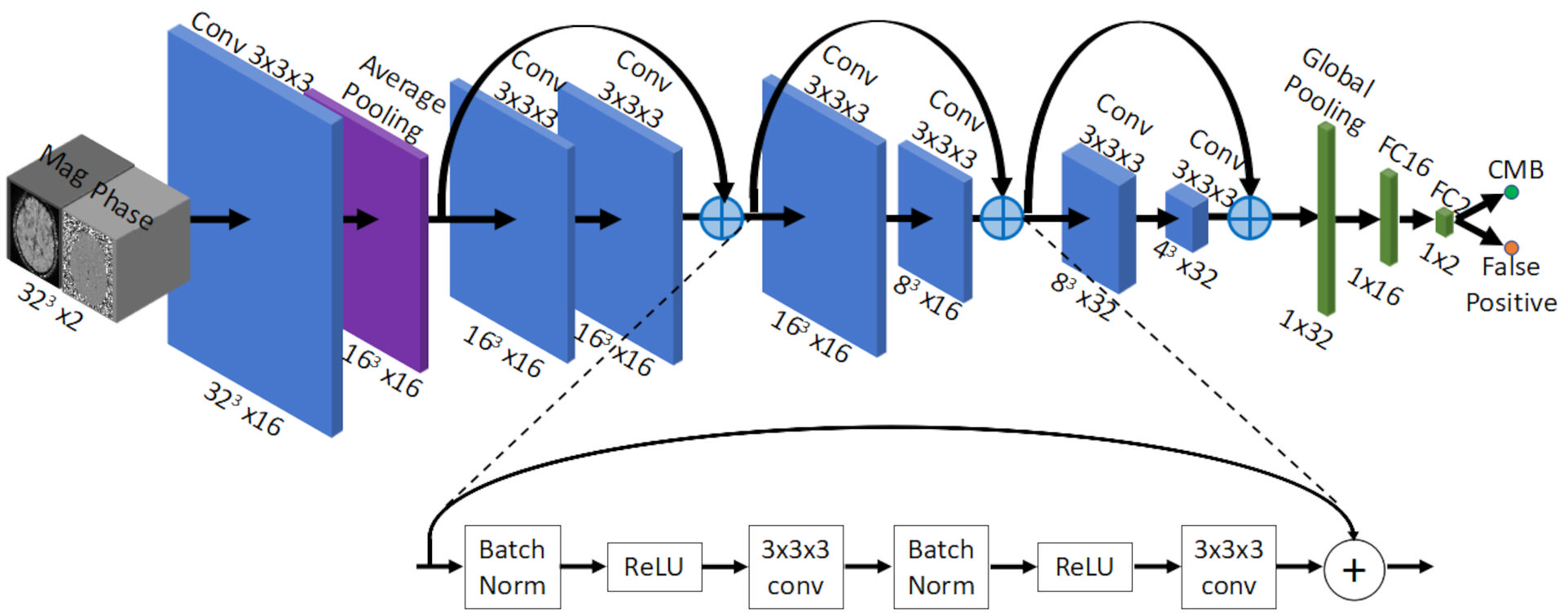
The whole pipeline has two major components: 1) CMB candidate detection and 2) false positive reduction. For step 1, candidates were selected by thresholding the 3D fast radial symmetry transformed (3D-FRST) SWI magnitude images [5]. For each candidate, 3D volumes were cropped from different types of images, and were input to step 2. For step 2, we designed a deep learning architecture based on residual networks (Figure 1) for binary classification (0: false positive, 1: true CMB). Training was performed on a desktop equipped with 24G RAM and a NVIDIA GTX-1080ti GPU. Different combinations of the input image types were tested. For each type of input, four models were selected based on the performance on the training and validation data. Data were collected using conventional SWI sequences on 1.5T and 3T scanners, including 13 stroke cases, 97 traumatic brain injury (TBI) cases, 100 hemodialysis cases, and 10 normal controls. The data pre-processing steps included bias-field correction [6], generating susceptibility maps [7] and interpolation to 0.5mm isotropic resolution. The training was performed on 3072 samples (from 154 subjects) and the performance of the model was monitored on 480 validation samples (from 25 subjects). Both the conventional CMBs (e.g., those in stroke and hemodialysis cases) and bleeds connected with vessels (e.g., those in TBI cases) were labeled as 1, while randomly sampled background regions, normal veins and iron deposition regions in basal ganglia structures were labeled as 0. Finally, the model was tested on 41 cases (TBI: 9, stroke: 9, hemodialysis: 13 and healthy controls: 10), and compared with three human raters. The gold standard in the test data were obtained based on the consensus of all three raters.Results
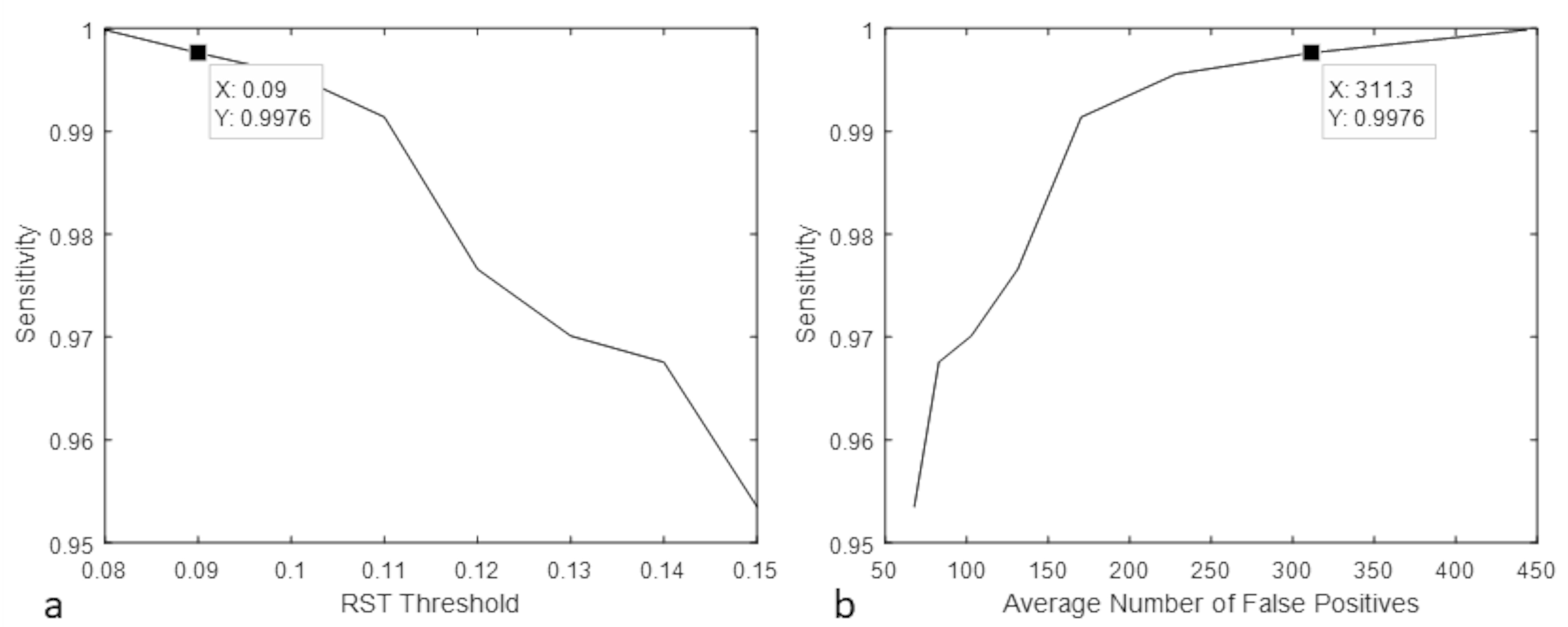
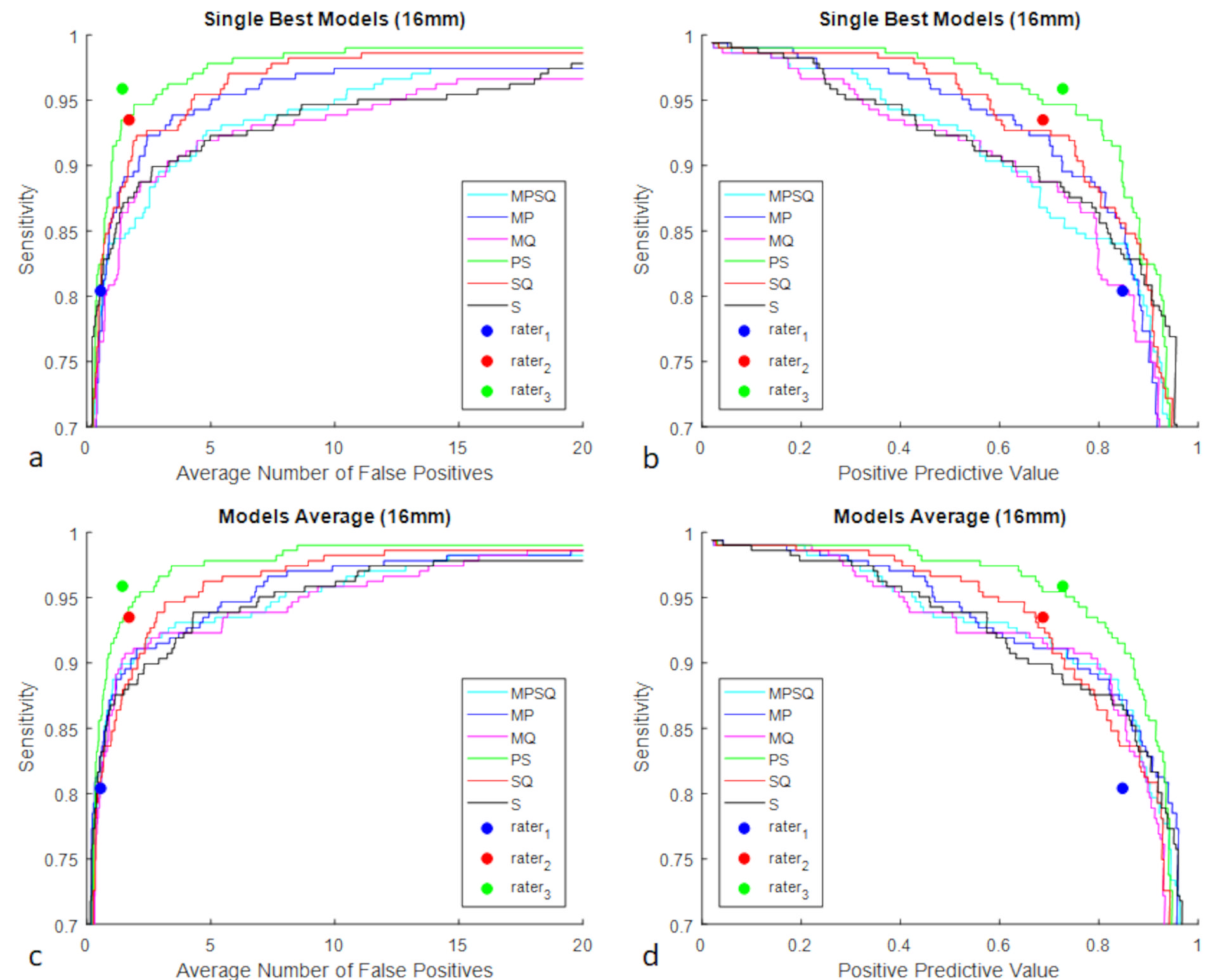
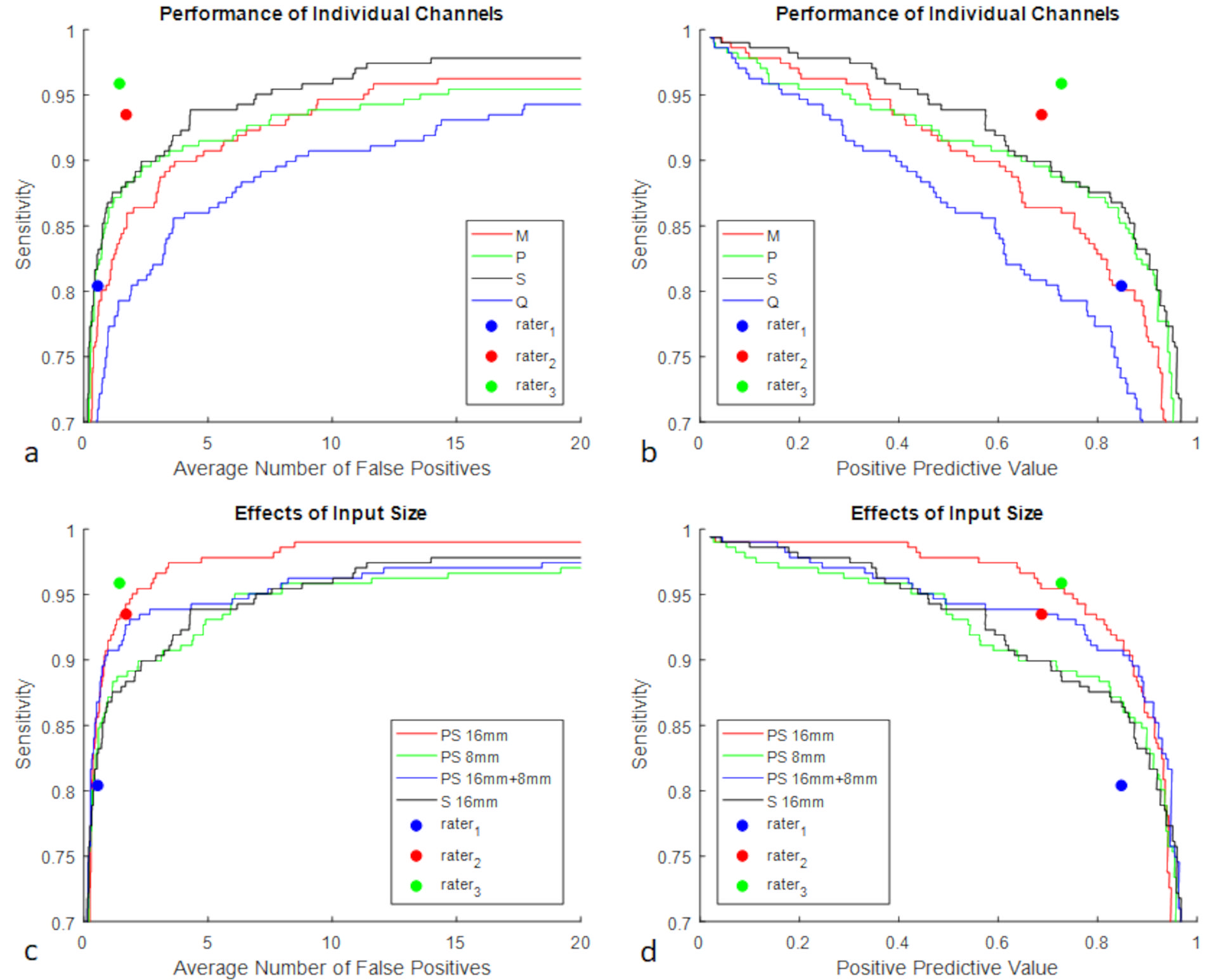
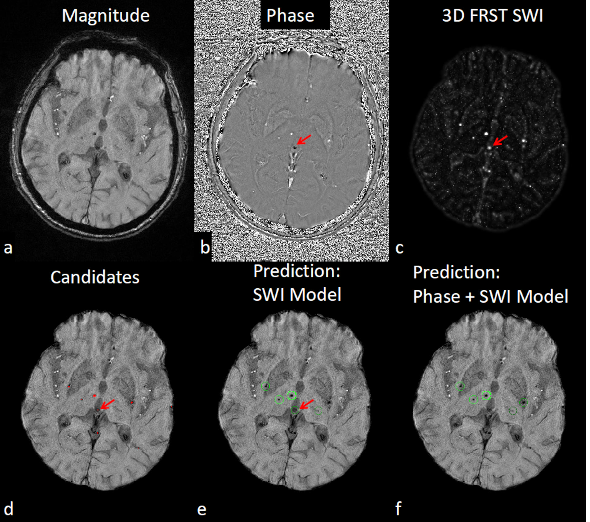
CMB candidates detection: With 3D-RST and a threshold=0.09, a sensitivity of 99.8% was achieved with the average number of false positives (FPavg) being 311.3 for the train and validation data (Figure 2). On the test data, it was found that the sensitivity was 99.4%, with FPavg being 286.3 in the detected candidates. False positive reduction: Figure 3 shows the performance of single models with different types of input. The combination of phase and SWI outperformed all the other models. The average of phase + SWI models had similar performance to rater 3 (senior SWI data processor), and outperformed both rater 1 (SWI data processor) and rater 2 (radiologist). Figure 4 shows that the largest input size (16mm) performed the best. SWI was found to be the most useful image, followed by phase, magnitude and QSM. However, using SWI alone, the false positives caused by calcification were not removed. Phase +SWI models successfully eliminated that false positive (red arrow in Figure 5). Among all three raters, rater 3 performed the best, with sensitivity 96%, positive predictive value (PPV) 73%, and FPavg 1.5. At the same level of FPavg, the sensitivity and PPV of the phase+SWI model was 93% and 80%, respectively. This is significantly better than the model using SWI alone, as reported by Dou et al., 2016 : sensitivity: 93%, PPV: 44%, FPavg: 2.74 [3].Discussion and Conclusion
In this study, we developed a deep learning model for CMB detection using 3D multi-contrast SWI data. The use of phase images together with SWI magnitude images significantly improved the performance over models using SWI magnitude images alone. QSM was not found to add much value, possibly be due to the loss of phase information caused by high-pass filtering of the original phase images. Our model outperformed the previously reported SWI based deep learning models and achieved similar performance to the most experienced human rater. This study has demonstrated the potential of applying deep learning to radiologic diagnostic MR imaging.Acknowledgements
The authors would like to thank Dr. Yi Zhong, Ying Wang and Sean Sethi for their insightful comments.References
1. Liu S, Buch S, Chen Y, Choi H-S, Dai Y, Habib C, Hu J, Jung J-Y, Luo Y, Utriainen D, Wang M, Wu D, Xia S, Haacke EM. Susceptibility-weighted imaging: current status and future directions. NMR Biomed. 2017;30.
2. Barnes SRS, Haacke EM, Ayaz M, Boikov AS, Kirsch W, Kido D. Semiautomated detection of cerebral microbleeds in magnetic resonance images. Magn. Reson. Imaging 2011;29:844–52.
3. Qi Dou null, Hao Chen null, Lequan Yu null, Lei Zhao null, Jing Qin null, Defeng Wang null, Mok VC, Lin Shi null, Pheng-Ann Heng null. Automatic Detection of Cerebral Microbleeds From MR Images via 3D Convolutional Neural Networks. IEEE Trans. Med. Imaging 2016;35:1182–95.
4. He K, Zhang X, Ren S, Sun J. Deep Residual Learning for Image Recognition. The IEEE Conference on Computer Vision and Pattern Recognition (CVPR), 2016, pp. 770-778
5. Loy G, Zelinsky A. A Fast Radial Symmetry Transform for Detecting Points of Interest. In: Heyden A, Sparr G, Nielsen M, Johansen P, editors. Computer Vision — ECCV 2002. Springer Berlin Heidelberg; 2002. page 358–68.
6. N.J. Tustison, B.B. Avants, P.A. Cook, Y. Zheng, A. Egan, P.A. Yushkevich, J.C. Gee, N4ITK: improved N3 bias correction, Medical Imaging IEEE Transactions on, vol. 29, no. 6, pp. 1310-1320, 2010.
7. Haacke EM, Liu S, Buch S, Zheng W, Wu D, Ye Y. Quantitative susceptibility mapping: current status and future directions. Magn Reson Imaging. 2015 Jan;33(1):1-25. doi: 10.1016/j.mri.2014.09.004.
Figures