Synopsis

We propose an enhanced recursive residual network (ERRN) that improves the basic recursive residual network with both a high-frequency feature guidance and dense connections. The feature guidance is designed to predict the underlying anatomy based on image a priori learning from the label data, playing a complementary role to the residual learning. The ERRN is adapted to include super resolution MRI and compressed sensing MRI, while an application-specific error-correction unit is added into the framework, i.e. back projection for SR-MRI and data consistency for CS-MRI due to their different sampling schemes.

INTRODUCTION

METHODS

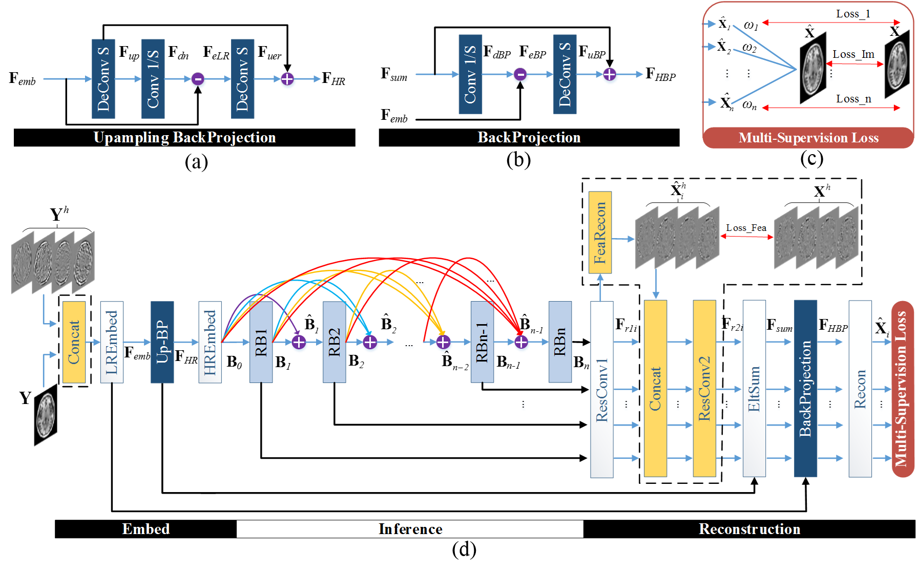
The basic architecture of our recursive residual network consists of three subnetworks: an embedding net, an inference net and a reconstruction net as shown in Fig.1. The embedding net is employed to extract structure features from the low quality image. The inference net is stacked by a set of parameter-shared residual blocks, on which training is executed in a multi-supervision strategy. Feature maps output from every residual block are convolved in the reconstruction net and then summed up in the EltSum layer. Consequently, the intermediate prediction $$$\bf{\widehat{X_{\it{i}}}}$$$ of each residual block is involved in weighted averaging $$$\bf\widehat{X}=\sum_\it{i}^\it{n}\omega_{i}\widehat{{\bf{X}}_{i}}$$$, using the part of Multi-Supervision Loss.

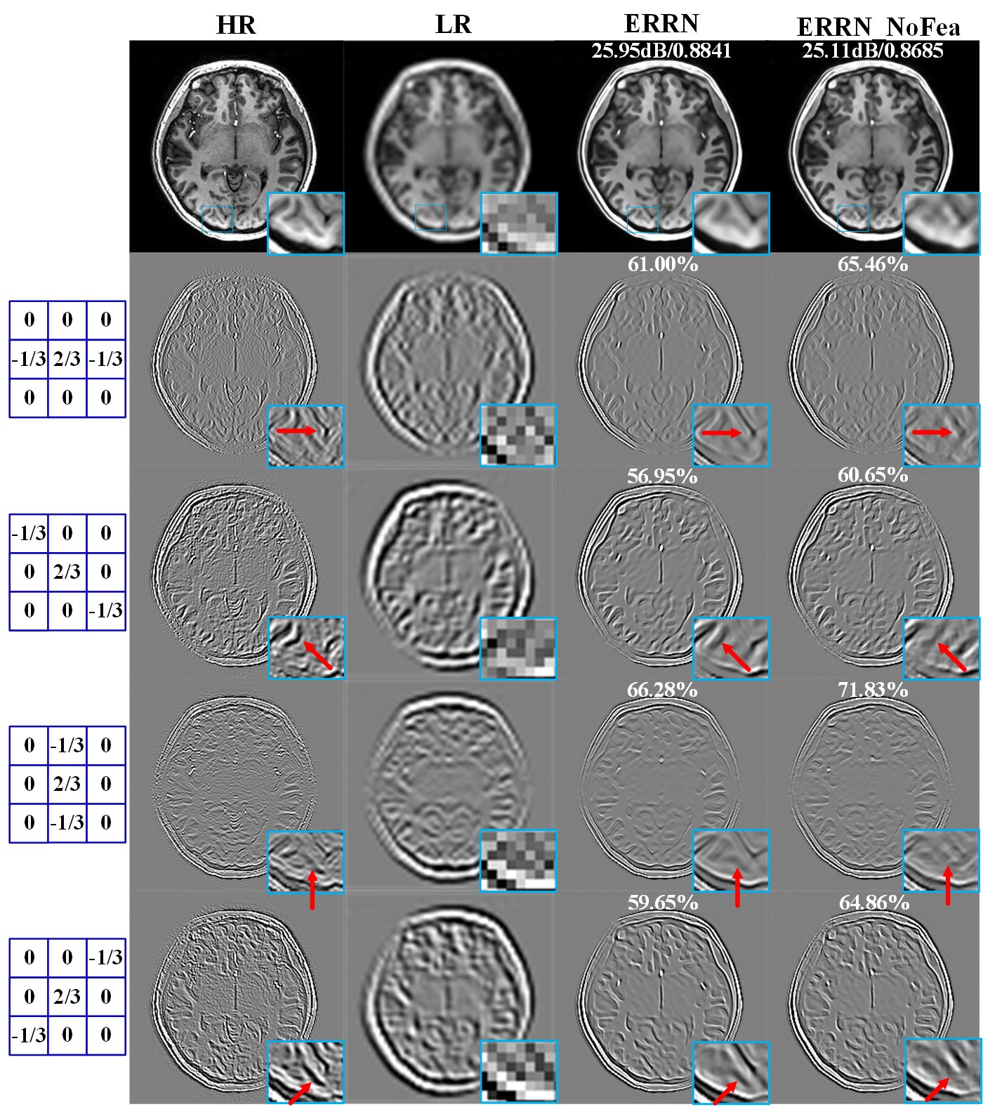
We create four directional filters G and detect structural features from undersampled data and corresponding label images using $$$\bf Y^{\it{h}}=G{\otimes}Y$$$ and $$$\bf X^{\it{h}}=G{\otimes}X$$$, shown in Fig.2. The low quality images Y and their structural features Y^h are concatenated as the network input. Besides, the primary feature guidance module is inserted in the reconstruction net, outlined by dashed borders in Fig. 1. In this way, feature maps generated from B_i are convolved in ResConv1 layer, and then flow into the FeaRecon layer to predict the underlying anatomy supervised by feature priori X^h. The learned features $$${\bf \widehat{X}}_i^h$$$ are fed back to the main framework.

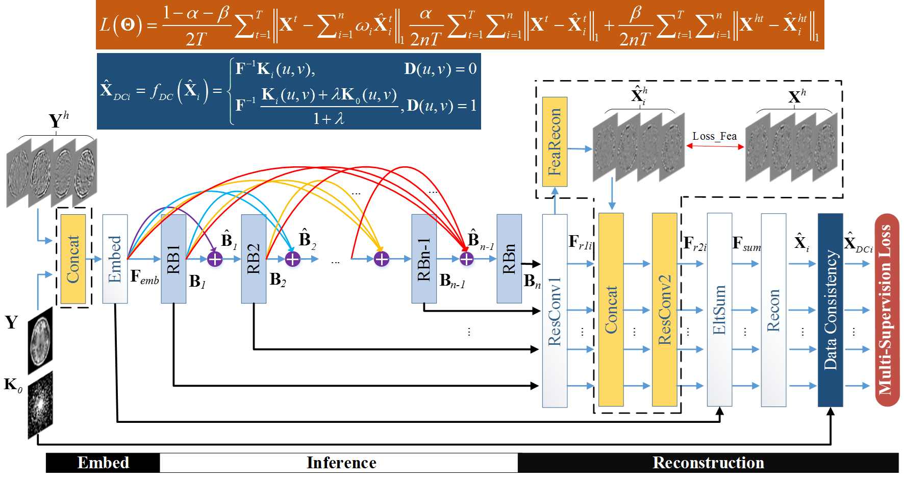
Although the SR- and CS-MRI are common undersampling problems in medical imaging, their sampling schemes are different in that one is uniform and the other random. In that regard, our network is further enhanced with application specific error-correction units. In Fig.1, the back projection^3,4 for SR-MRI is composed of an upsampling layer Up-BP and another BackProjection layer. In Fig.3, the CS-MRI framework shares mostly the same architecture as SR-MRI, except that a data consistency⁵ unit is used in ERRN for CS-MRI.

RESULTS

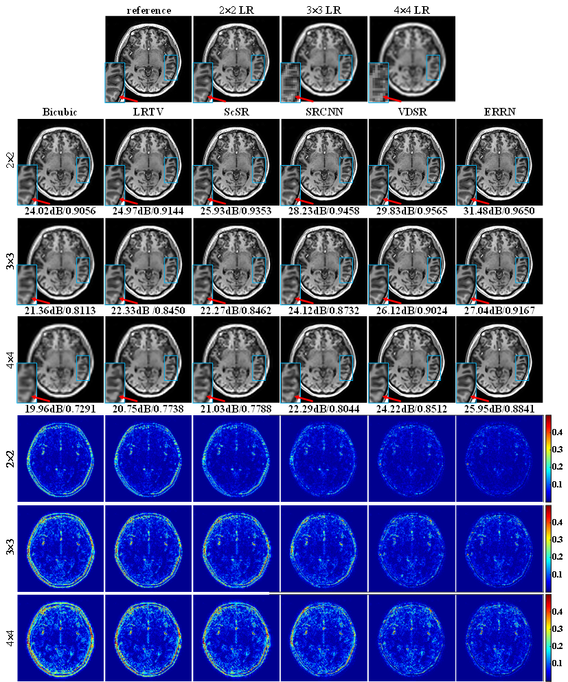
Fig. 4 shows SR-MRI reconstruction results in the T1-weighted adult brain associated with their PSNR and SSIM values. We can see that the CNN-based methods have remarkable improvements over the optimization-based methods of LRTV⁶ and ScSR⁷. The deep networks of VDSR⁸ and ERRN achieve superior performances compared to the simple SRCNN⁹. Moreover, proposed ERRN takes advantage of fine tissue structures and high image quality accompanied with a remarkable increase in PSNR and SSIM, particularly for an undersampling rate of more than 10-fold. The ERRN reconstruction time is 0.06s.

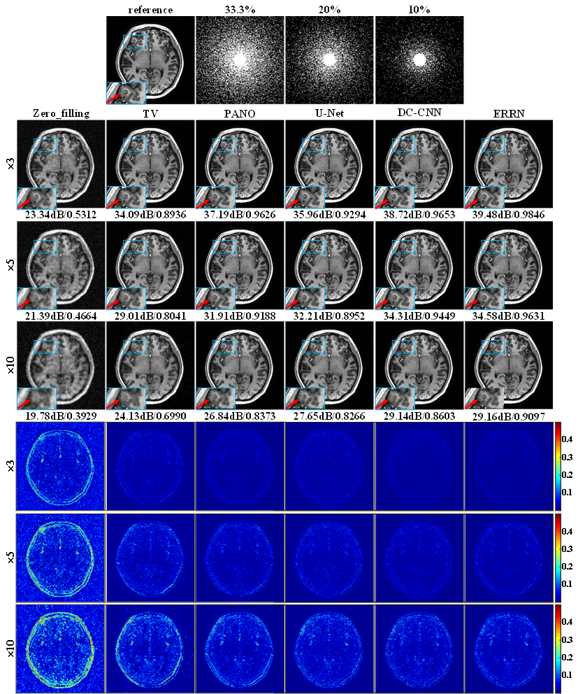
Fig.5 shows CS-MRI reconstruction results for the same slice as used for SR-MRI, where the traditional zero-filling, TV method¹⁰ and PANO¹¹ were exploited, as well as deep networks of U-net¹² and DC-CNN⁵. In general, the ERRN achieved the best performance at all acceleration rates with highest PSNR and SSIM values. The reconstructions with DC-CNN and ERRN are comparable in terms of PSNR, whereas the ERRN result shows higher SSIM and the DC-CNN result is somewhat over-smoothed. This is in agreement with the expectations that anatomy structures can be distinctly restored by ERRN thanks to the feature guidance.

DISCUSSION

In ERRN, we have more control on the “black box” operations of the deep learning, which is meaningful for the application-specific network to avoid over-fitting and achieve improved performance. We have performed an effect analysis for different modules, i.e. the feature guidance, the dense connections, the back projection and the data consistency. Results demonstrated that every module shows noticeable impact on the converge curve. We determined the number of residual block n=10 in our ERRN experiments, which is a trade-off between the network complexity, the reconstruction performance and the training time. The time efficiency of ERRN is comparable to other networks of similar depth but less parameters, almost over 100 times faster than optimization-based methods, making it more feasible for real-time reconstruction on MRI scanners.

Our network was implemented in TensorFlow with ADAM optimizer on a Linux workstation with Intel Xeon processors E5-2620, 12GB NVIDIA Pascal Titan X and 64GB RAM. The brain dataset contained 440 two-dimensional images acquired at a 7T scanner. We selected 10% data for testing, whereas the remainder were used for training with data augmentation. The network learning rate was 10^-4 and gradually converged after 50 epochs.

Acknowledgements

References

[1] J. Kim, J. Kwon Lee, and K. Mu Lee, “Deeply-recursive convolutional network for image super-resolution,” in Proc. IEEE CVPR, Las Vegas, NV, USA, 2016, pp. 1637-1645.

[2] K. He, X. Zhang, S. Ren, and J. Sun, “Deep residual learning for image recognition,” in Proc. IEEE CVPR, Las Vegas, NV, USA, 2016, pp. 770-778.

[3] M. Haris, G. Shakhnarovich, and N. Ukita, “Deep back-projection networks for super-resolution,” in Proc. IEEE CVPR, Salt Lake City, USA, 2018, pp. 1664-1673.

[4] E. V. Reeth, I. W. K. Tham, C. H. Tan, and C. L. Poh, “Super-resolution in magnetic resonance imaging: A review,” Concept. Magn. Reson. A, vol. 40A, no. 6, pp. 306-325, Nov. 2012.

[5] J. Schlemper, J. Caballero, J. V. Hajnal, A. Price, and D. Rueckert, “A deep cascade of convolutional neural networks for dynamic MR image reconstruction,” IEEE Trans. Med. Imag., vol. 37, no. 2, pp. 491-503, Feb. 2018.

[6] S. Feng, C. Jian, W. Li, P. T. Yap, and D. Shen, “LRTV: MR image super-resolution with low-rank and total variation regularizations,” IEEE Trans. Med. Imag., vol. 34, no. 12, pp. 2459-2466, Jun. 2015.

[7] J. Yang, J. Wright, T. S. Huang, and Y. Ma, “Image super-resolution via sparse representation,” IEEE Trans. Image Process., vol. 19, no. 11, pp. 2861-2873, Nov. 2010.

[8] J. Kim, J. Kwon Lee, and K. Mu Lee, “Accurate image super-resolution using very deep convolutional networks,” in Proc. IEEE CVPR, Las Vegas, NV, USA, 2016, pp. 1646-1654.

[9] C. Dong, C. C. Loy, K. He, and X. Tang, “Image super-resolution using deep convolutional networks,” IEEE Trans. Pattern Anal. Mach. Intell., vol. 38, no. 2, pp. 295-307, Feb. 2016.

[10] M. Lustig, D. Donoho, and J. Pauly, “Sparse MRI: The application of compressed sensing for rapid MR imaging,” Magn. Reson. Med., vol. 58, no. 6, pp. 1182-1195, Dec. 2007.

[11] X. Qu, Y. Hou, F. Lam, D. Guo, J. Zhong, and Z. Chen, “Magnetic resonance image reconstruction from undersampled measurements using a patch-based nonlocal operator,” Med. Image Anal., vol. 18, no. 6, pp. 843-856, Aug. 2014.

[12] O. Ronneberger, P. Fischer, and T. Brox, “U-net: Convolutional networks for biomedical image segmentation,” in Proc. MICCAI, Munich, Germany, 2015, pp. 234-241.