Synopsis

AUTOMAP is a promising generalized reconstruction approach, however, it is not scalable and hence the practicality is limited. We present a novel way for decomposing the domain transformation, which makes the model scale linearly with the input size. We show the proposed method, termed dAUTOMAP, outperforms AUTOMAP with significantly fewer parameters.

Introduction

Recently, automated transform by manifold approximation (AUTOMAP)^[1] has been proposed as an innovative approach to directly learn the transformation from source signal domain to target image domain. While the applicability of AUTOMAP to a range of tasks has been demonstrated, its practicality remains limited as the required number of parameters scales quadratically with the input size. We present a novel way for decomposing the domain transformation, which makes the model scale linearly with the input size. We term the resulting network dAUTOMAP (decomposed - AUTOMAP). We show that, remarkably, the proposed approach outperforms AUTOMAP for the provided dataset with significantly fewer parameters.

Methods

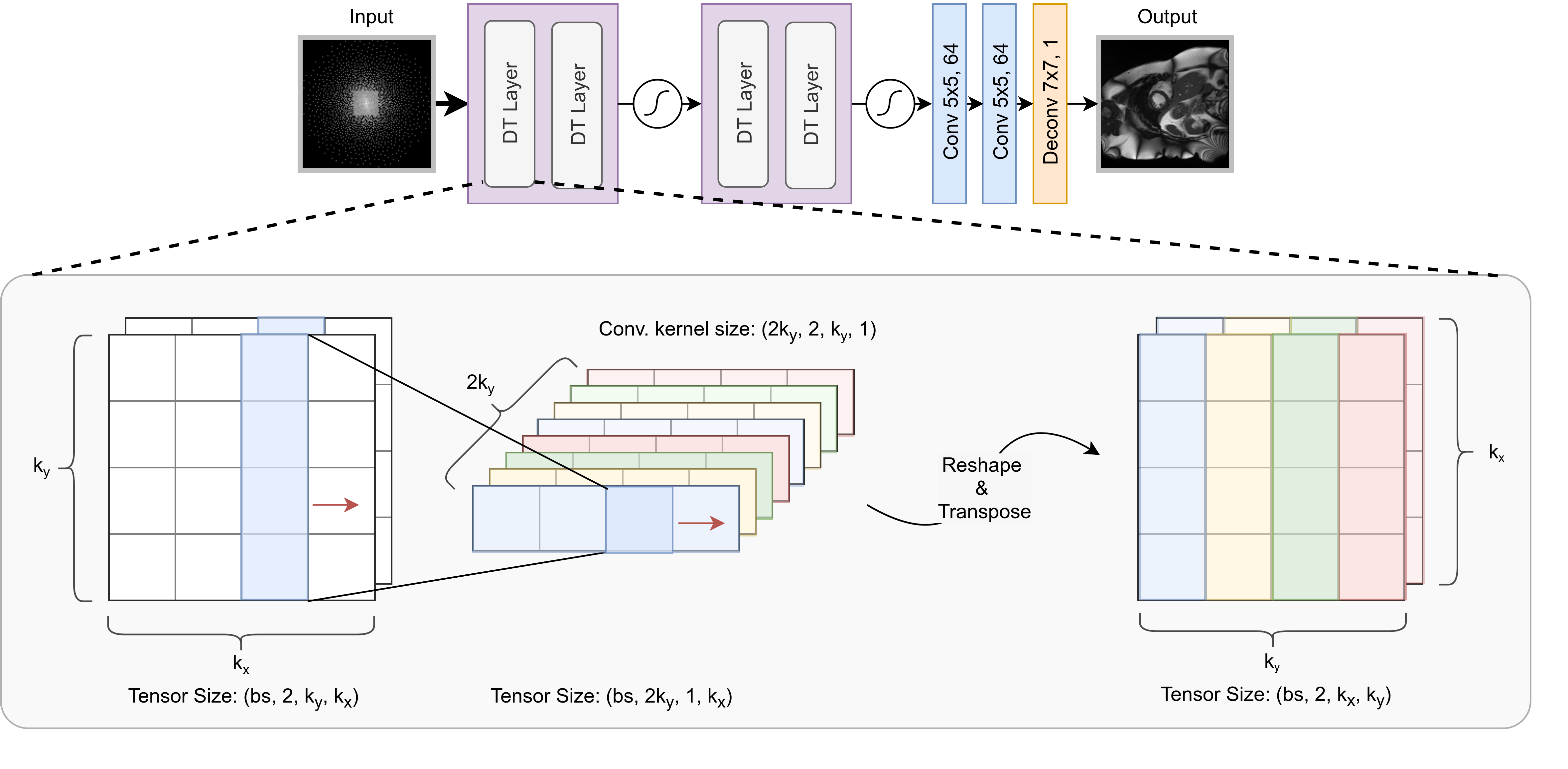
Let $$$\mathbf{x} \in \mathbb{C}^{N \times M}$$$ be a complex-valued image. The two-dimensional Discrete Fourier Transform (DFT) is given by:\begin{align} \mathbf{y}[k, l] = \sum_{n=0}^{N} \sum_{m=0}^{M} \mathbf{x} [n, m] e^{-j2\pi \left( \frac{nk}{N} + \frac{ml}{M} \right)}. \end{align}This is commonly written as a matrix product: $$$ \text{vec}(\mathbf{y}) = \mathbf{E} \text{vec}(\mathbf{x}) $$$, where we take row-order vectorization and $$$\mathbf{E}_{pq} = e^{-j2\pi \left( \frac{nk}{N} + \frac{ml}{M} \right)}$$$, with $$$p = kM + l$$$, $$$q = nM + m$$$. As the matrix $$$\mathbf{E}$$$ is the Kronecker product of two one-dimensional DFT’s, we have:$$ \mathbf{E} \text{vec}( \mathbf{x} ) = \left( \mathbf{F}_N \otimes \mathbf{F}_M \right) \text{vec}( \mathbf{x} ) = \text{vec}( \mathbf{F}_N \mathbf{x} \mathbf{F}_M^H ) = \text{vec} \left( \left( \mathbf{F}_M ( \mathbf{F}_N \mathbf{x} )^H \right)^H \right),$$where $$$(\mathbf{F}_N)_{kn} = e^{-j2\pi \frac{nk}{N} }, (\mathbf{F}_M)_{lm} = e^{-j2\pi \frac{ml}{M} }$$$. Observe that $$$\mathbf{F}_N \mathbf{x}$$$ can be computed using a convolution layer with $$$N$$$ kernels of size $$$(N,1)$$$ with no padding where the output tensor has size $$$(N_\text{batch}, N, 1, M)$$$. Motivated by this, we propose a decomposed transform layer (DT layer): a convolution layer with the above kernel size, which is learnable. In the simplest case, the layer can be reduced to the (inverse) Fourier transform or identity. A 2D DFT can be performed by applying the DT layer twice, where the intermediate tensor is first reshaped into $$$(N_\text{batch}, 1, N, M)$$$ and then conjugate-transposed. Note that the complex nature of the operation is preserved by $$$\mathbb{R}^2$$$, which doubles the number of output channels (i.e. $$$2N$$$).Therefore, the convolution kernel of the DT layer has the shape: $$$(N_{c_{out}}, N_{c_{in}}, \text{kernel}_x, \text{kernel}_y) = (2N, 2, N, 1)$$$. For the second DT layer, N and M are swapped.

The proposed dAUTOMAP, shown in Figure 1, replaces the fully-connected layers in AUTOMAP by DT layers. We used ReLU as the choice of non-linearity.

Evaluation

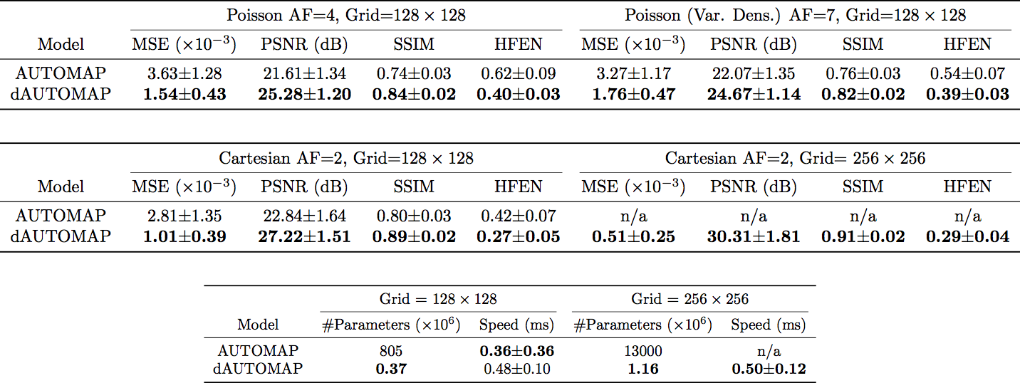
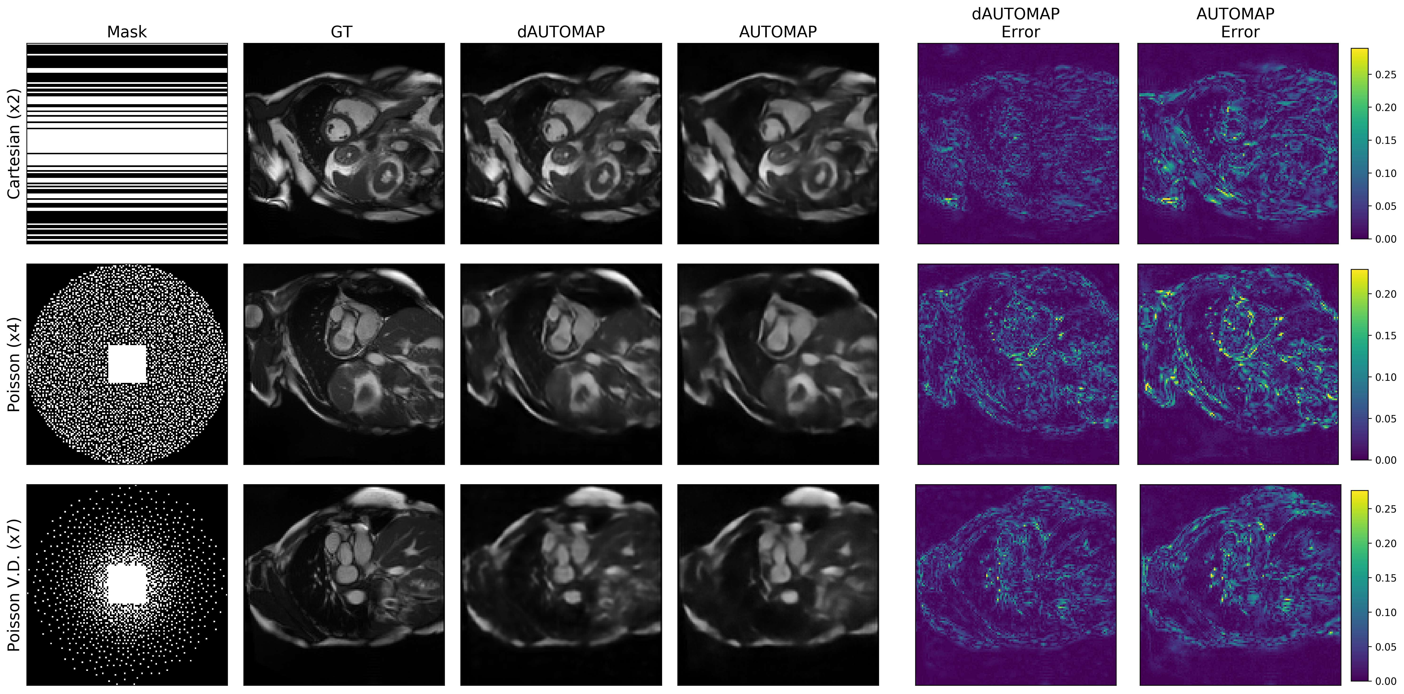
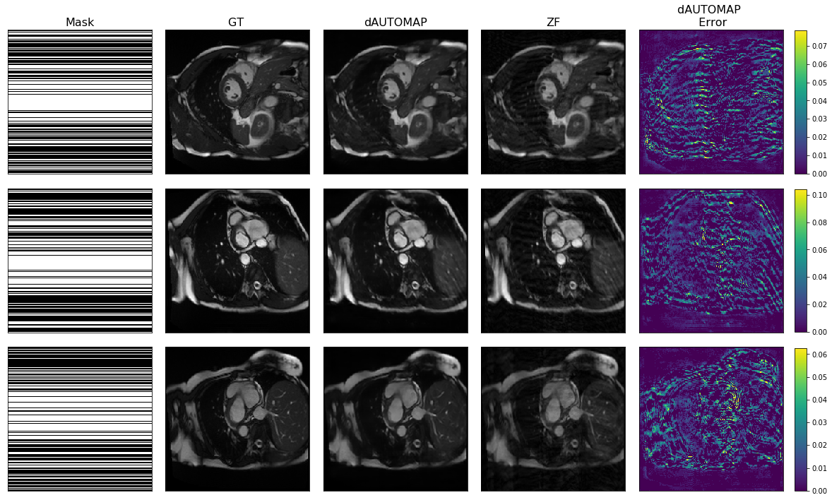
We evaluated the proposed method on a simulation-based study using short-axis (SA) cardiac cine magnitude images from the UK Biobank Study^[2] (>1M SA slices). To compare with AUTOMAP, the data were subsampled to central $$$128 \times 128$$$ $$$k$$$-space grid points. Both methods were evaluated on the reconstruction tasks from three undersampling patterns: (1) Cartesian with Acceleration Factor (AF) =2, (2) Poisson^[3] with AF=4, (3) Variable density Poisson with AF=7. For dAUTOMAP, we also experimented with the images having $$$256 \times 256$$$ $$$k$$$-space grid points, with $$$2\times$$$ Cartesian undersampling (such input size causes memory error for AUTOMAP). Both networks were initialised randomly and trained for 1000 epochs to minimise the standard $$$\ell_2$$$ loss with batch size 128. We used RMSProp with $$$lr=2 \times 10^{-5}$$$ and Adam optimiser $$$lr=10^{-3}$$$ for AUTOMAP and dAUTOMAP respectively. The reconstructions were evaluated by mean squared error (MSE), peak signal-to-noise ratio (PSNR), structural similarity (SSIM) and High Frequency Error Norm (HFEN). We also compared the reconstruction speed and the required parameters.

Results

As shown in Figure 2, the proposed approach outperformed AUTOMAP (Wilcoxon, $$$p \ll 0.01$$$). Figure 3-4 shows sample reconstructions. We notice that AUTOMAP tends to over-smooth the image, whereas dAUTOMAP preserves the fine-structure better, even though the residual artefact is more prominent. The result of dAUTOMAP for $$$256 \times 256$$$ $$$k$$$-space data is shown in Figure 5, demonstrating that the method successfully learnt a transform which simultaneously dealiases the image. The execution speeds were comparable. The parameters of the proposed approach required only 1.5MB of memory for $$$128 \times 128$$$ $$$k$$$-space data, compared to 3.1GB required for AUTOMAP (these numbers increase to 3.1MB vs. 56GB for $$$256 \times 256$$$ $$$k$$$-space data).

Discussion and Conclusion

Acknowledgements

References

[1] Zhu, Bo, et al. "Image reconstruction by domain-transform manifold learning." Nature 555.7697 (2018): 487.

[2] Petersen, Steffen E., et al. "UK Biobank’s cardiovascular magnetic resonance protocol." Journal of Cardiovascular Magnetic Resonance 18.1 (2015): 8.

[3] BART Toolbox for Computational Magnetic Resonance Imaging, DOI: 10.5281/zenodo.592960