0596
Differential Diagnosis of Benign and Malignant Breast Lesions Based on DCE-MRI by Using Radiomics and Deep Learning with Five Different NetworksJiejie Zhou1, Yang Zhang2, Kai-Ting Chang2, Peter Chang2, Daniel Chow2, Ouchen Wang3, Meihao Wang1, and Min-Ying Lydia Su2
1Department of Radiology, The First Affiliate Hospital of Wenzhou Medical University, Wenzhou, China, 2University of California, Irvine, CA, United States, 3Department of Thyroid and Breast Surgery, The First Affiliate Hospital of Wenzhou Medical University, Wenzhou, China
Synopsis
A total of 152 patients receiving breast MRI for diagnosis were analyzed, including 93 patients with 103 malignant cancers, and 59 patients with 73 benign lesions. Three DCE parametric maps corresponding to early wash-in, maximum, and wash-out were generated. Radiomics analysis based on texture and intensity histogram, and deep learning using 5 networks, were performed for differential diagnosis. The accuracy of radiomics was 0.80, and the accuracy of deep learning varied in the range of 0.79-0.94 depending on the network. The smallest bounding box containing the tumor with small amount of per-tumor tissue has the highest diagnostic accuracy.
Introduction
Breast MRI is an important clinical imaging modality for screening, diagnosis and pre-operative staging of breast cancer. With the improved technology, automatic and quantitative analysis of detected lesion may provide important information. Dynamic contrast enhanced MRI (DCE-MRI) can achieve a high sensitivity; however, it also detects many benign lesions. Such incidental findings may bring anxiety to patients and also lead to unnecessary biopsies or over treatment. With more and more screening and preoperative MRI performed, a better characterization of the enhancing lesions detected by MRI is important to improve diagnostic accuracy. Other than evaluation based on radiologists’ visual assessment, radiomics using computer algorithms can extract comprehensive quantitative features to characterize lesion and develop diagnostic models. Recently, deep learning methods, especially Convolution Neural Network, are extensively applied for medical image processing, which can be used for tumor diagnosis as well. The goal of this study is to evaluate and compare the diagnostic accuracy of breast lesions detected on MRI using radiomics and deep learning with 5 different convolutional neural networks.Methods
A total of 152 patients were included in this study, including 93 patients with a total of 103 pathologically confirmed malignant cancers (mean age 52±11), and 59 patients with a total of 73 benign lesions diagnosed by pathological confirmation or follow-up (mean age 45±9). The MRI was performed using a GE 1.5T system. DCE was acquired using 6 frames, one pre-contrast (F1) and 5 post-contrast (F2-F6). Tumors were segmented based on contrast-enhanced maps using computer algorithms. For mass tumors, fuzzy-C-means (FCM) clustering algorithm was applied [1]. Figures 1-2 show two case examples, one malignant invasive ductal cancer and one benign fibroadenoma, respectively. For non-mass lesions, the FCM did not work well, and region growing was used to obtain the tumor boundary. Three heuristic DCE parametric maps were generated according to: the early wash-in signal enhancement (SE) ratio [(F2-F1)/F1]; the maximum SE ratio = [(F3-F1)/F1]; the wash-out slope [(F6-F3)/F3] [2]. For radiomics analysis, the segmented tumor on each map was analyzed to obtain 12 histogram parameters and 20 GLCM texture features [3]. For differentiation between benign and malignant lesions, the random forest algorithm was used to select features with the highest significance [4], and then these features were used to train a logistic model to serve as a classifier. The deep learning was performed by using 5 different convolutional neural networks, including ResNet50 [5], VGG16 [6], VGG19 [6], Xception [7], and InceptionV3 [8]. The analysis was done based on three DCE parametric maps. For each case, the smallest square bounding box containing the entire tumor was generated. To increase the case number, all slices were used as independent inputs, and the dataset was further augmented by random affine transformation. The loss function is cross entropy and the optimizer is Adam with learning rate 0.001 [9]. ImageNet works as the initial values of the parameters in these models [10]. The accuracy was evaluated using 10-fold cross-validation. To evaluate the role of peritumoral environment, the analysis was done using 5 different input methods: 1) the tumor ROI only by setting all outside tumor pixels in the box as zero, 2) the smallest bounding box, 3) enlarged by 1.2 times, 4) enlarged by 1.5 times, and 5) enlarged by 2 times. The box was resized to 64x64 as input in deep learning. The obtained results were compared.Results
The DCE time course measured from the segmented tumor in Figures 1 and 2 are shown in Figure 3. The kinetic pattern of invasive ductal cancer is a typical wash-out pattern, reaching maximum in the second post-contrast frame (F3), and then showing decreased signal intensity in frames F4 to F6. The benign fibroadenoma also demonstrates strong contrast enhancement, and the DCE kinetics shows a persistent enhancement pattern with increasing intensity from F1 to F6. The radiomics analysis achieves the highest classification accuracy of 0.8. For deep learning, Table 1 summarizes the performances of 5 CNN models with 5 different inputs by selecting different sizes of bounding box. The results show that the smallest bounding box containing the tumor works the best for all CNN models. The mean accuracy of ResNet50 (0.93), Xception (0.94) and InceptionV3 (0.93) are better than the performance of VGG16 (0.80) and VGG19 (0.79).Discussion
Despite using a relatively large number of cases, the conventional radiomics based on histogram and texture features only achieved accuracy of 0.80. When using deep learning, the accuracy was higher, but it varied substantially depending on the algorithm that was used. The Xception method could yield the highest accuracy of 0.94. Previous studies have shown that the peritumor environments contain useful information to aid in diagnosis. In this study we also used different sizes of bounding box as inputs in deep learning to evaluate their role. The results show that the smallest bounding box has a slightly better performance compared to using the tumor ROI alone, suggesting that the immediate peritumor tissue outside the tumor boundary can provide useful information to help diagnosis. As the size of the box increases, the performance becomes worse and worse, which might be in part due to lower input image resolutions into the neural networks and the information from the tumor is diluted. With larger diagnostic breast MRI datasets gradually becoming available, the performance using different computer algorithms can be thoroughly evaluated, not limited by the case number, and the results may be used to develop a fully automatic diagnostic tool that can be implemented for clinical use.Acknowledgements
This work was supported in part by the Natural Science Foundation of Zhejiang (No.LY14H180006) and NIH R01 CA127927.References
[1]. Nie K, Chen J-H, Hon JY, Chu Y, Nalcioglu O, Su M-Y. Quantitative analysis of lesion morphology and texture features for diagnostic prediction in breast MRI. Academic radiology. 2008;15(12):1513-1525. [2]. Lang N, Su M-Y, Hon JY, Lin M, Hamamura MJ, Yuan H. Differentiation of myeloma and metastatic cancer in the spine using dynamic contrast-enhanced MRI. Magnetic resonance imaging. 2013;31(8):1285-1291. [3]. Haralick RM, Shanmugam K. Textural features for image classification. IEEE Transactions on systems, man, and cybernetics. 1973(6):610-621. [4]. Ho TK. Random decision forests. Paper presented at: Document analysis and recognition, 1995., proceedings of the third international conference on1995. [5]. He K, Zhang X, Ren S, Sun J. Deep residual learning for image recognition. Paper presented at: Proceedings of the IEEE conference on computer vision and pattern recognition2016. [6]. Simonyan K, Zisserman A. Very deep convolutional networks for large-scale image recognition. arXiv preprint arXiv:14091556. 2014. [7]. Chollet F. Xception: Deep learning with depthwise separable convolutions. arXiv preprint. 2017:1610.02357. [8]. Szegedy C, Vanhoucke V, Ioffe S, Shlens J, Wojna Z. Rethinking the inception architecture for computer vision. Paper presented at: Proceedings of the IEEE conference on computer vision and pattern recognition2016. [9]. Kingma D, Ba J. Adam: A method for stochastic optimization. arXiv preprint arXiv:14126980. 2014. [10]. Deng J, Dong W, Socher R, Li L-J, Li K, Fei-Fei L. Imagenet: A large-scale hierarchical image database. Paper presented at: Computer Vision and Pattern Recognition, 2009. CVPR 2009. IEEE Conference on2009.Figures
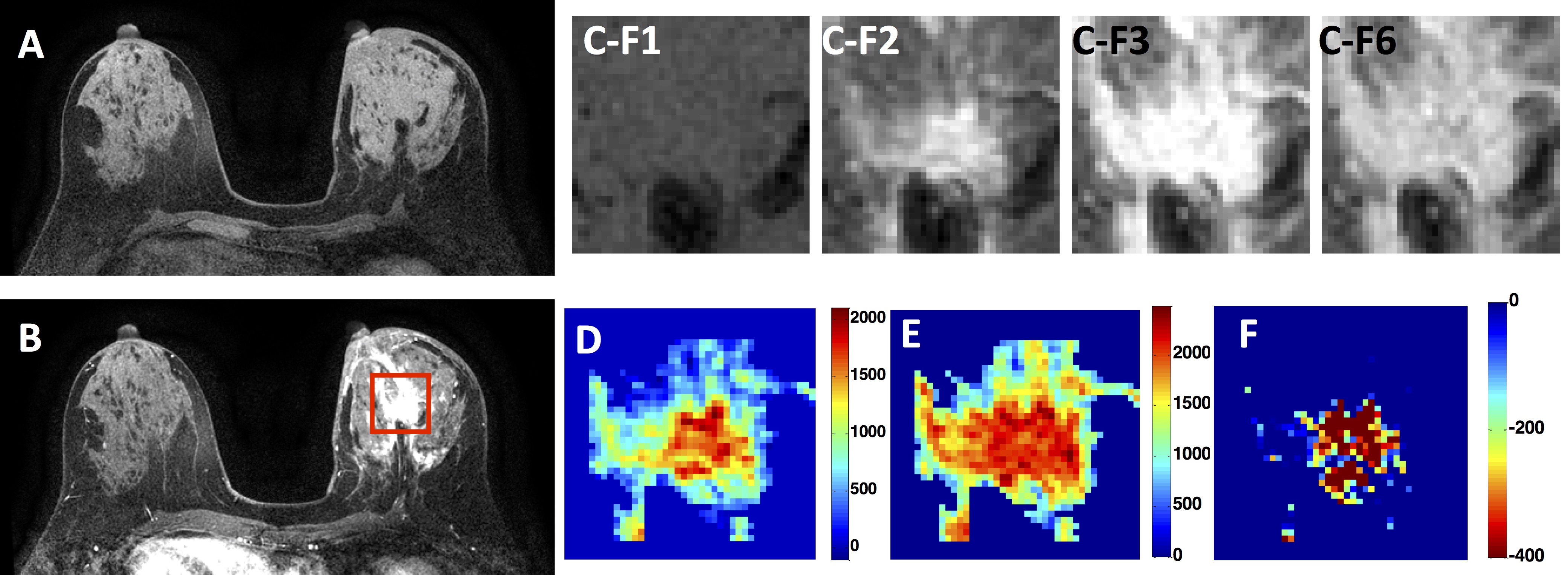
Figure
1: A 56-year-old patient with an irregular
malignant invasive ductal cancer that shows strong contrast enhancements. (A)
Pre-contrast image; (B) The 2nd post-contrast image (DCE Frame-3),
the red rectangle box is the smallest bounding box used as input in deep
learning analysis; (C) Four frames of pre- and post-contrast DCE
images (F1, F2, F3, and F6) of the smallest bounding box containing the tumor,
showing maximum enhancement in F3, and a clear wash-out in F6; (D) The early
wash-in signal enhancement map (F2-F1); (E) The maximum enhancement map
(F3-F1); (F) The wash-out Map (F6-F3), with most pixels showing negative
values. The DCE time course is shown in Figure 3A.
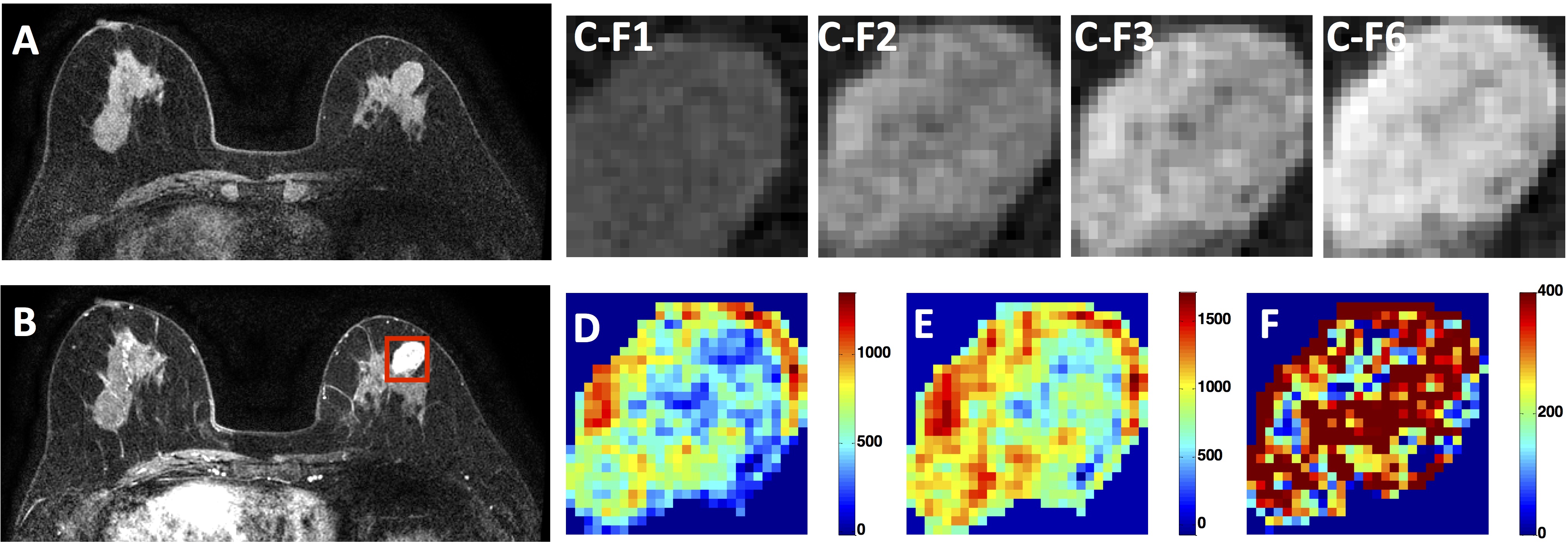
Figure
2: A
66-year-old patient with a benign fibroadenoma that shows strong contrast
enhancements with a smooth boundary. (A) Pre-contrast image; (B) The 2nd
post-contrast image (DCE Frame-3), the red rectangle box is the smallest
bounding box used as input in deep learning analysis; (C)
Four frames of pre- and post-contrast DCE images (F1, F2, F3, and F6) of the
smallest bounding box containing the tumor, showing persistent enhancements
over time; (D) The early wash-in signal enhancement map (F2-F1); (E) The
maximum enhancement map (F6-F1); (F) The wash-out Map (F6-F3). The DCE time
course is shown in Figure 3B.
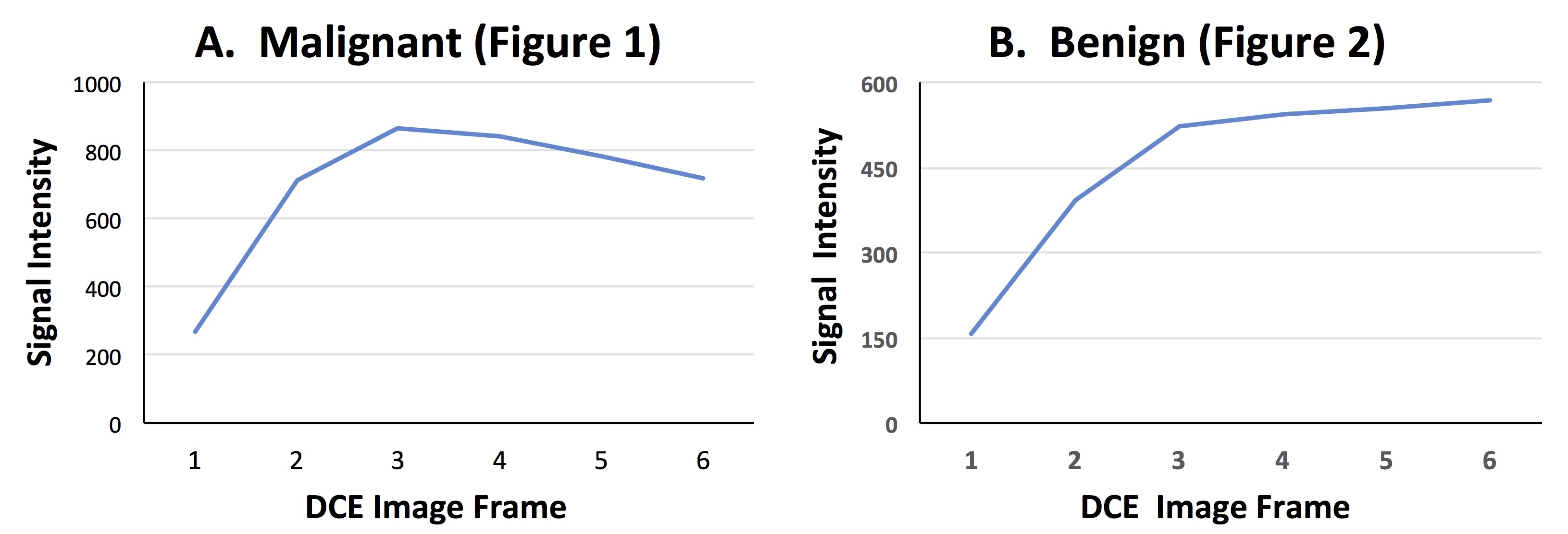
Figure
3: The DCE
time course of two cases. (A) The left curve corresponding to the Figure 1
patient with malignant invasive ductal carcinoma, showing a clear wash-out DCE
pattern. (B) The right curve corresponding to the Figure 2 patient with
benign fibroadenoma, showing a persistent enhancement DCE pattern with
continuously increasing enhancement over the DCE period.
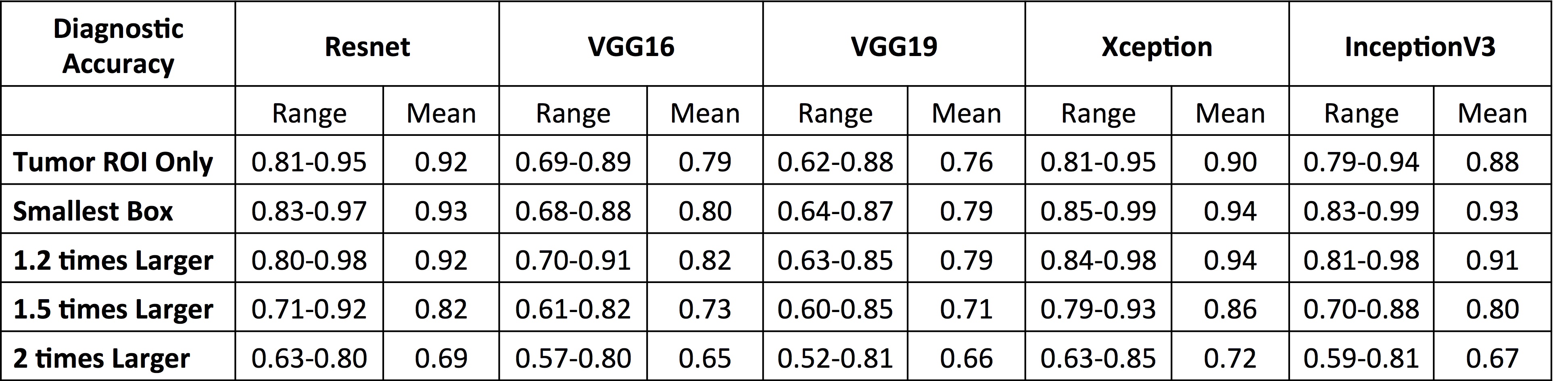
Table
1: The diagnostic accuracy analyzed using five
different deep learning algorithms, as well as the results obtained using
different sizes of bounding boxes as inputs.