0571
Fast and Intuitive RF-Coil Optimization Pipeline Using a Mesh-Structure1Center for Biomedical Imaging, Department of Radiology, NYU School of Medicine, New York, NY, United States, 2Center for Advanced Imaging Innovation and Research (CAI2R), NYU School of Medicine, New York, NY, United States
Synopsis
At the last years ISMRM we proposed an RF coil optimization pipeline based on a mesh structure consisting of 50-Ohm sources and copper patches. This allowed us to compute the maximal possible SNR of a given mesh as well as the emulation of concrete coil geometries in post-processing.
In this work we present an analysis of body imaging at 7T with an appropriately chosen mesh size that can reach the UISNR. Furthermore the optimal current weights are analyzed to create a physically realizable coil that approaches the UISNR.
Introduction
Traditional RF modelling methods can be used to make detailed analysis of RF coils. However, each new coil geometry under evaluation requires a dedicated simulation run. Alternatively, a generalized basis of EM fields could be used to compute the ultimate intrinsic SNR (UISNR) in a single simulation run1,2. Although such methods can provide valuable insights into the limits of RF coil design, it remains challenging to translate these findings into a specific physically realizable coil geometry.
In a first attempt, to bridge the gap between traditional
simulations and UISNR methods, we proposed a new RF coil optimization pipeline
based on a grid of dipoles, which allowed us to emulate different concrete coil
geometries in post-processing3. In this work, we extend our method to encompass
the UISNR and translate its current patterns to practical and physically
realizable coil designs.
Methods
As an example for the work-flow we chose to optimize a receive body coil for 7T. The optimization goal was chosen to be the central optimal SNR. For an easy comparison with respect to the UISNR and a more intuitive analysis we chose a cylindrical homogeneous phantom.
Three different sets of simulations were performed: the computation of the UISNR, the simulation of the mesh-structure and optimal coil array candidates. These coil candidates were chosen based on the analysis of the optimal currents of the mesh structure presented in the 'Results and Discussion' section.
The cylindrical phantom has body like properties ($$$R=20cm$$$,$$$\epsilon_r=32$$$,$$$\sigma=0.33S/m$$$,$$$L=1.3m$$$). The coil conductors are 5mm from the surface of the phantom. The numerical domain was terminated with an RF-shield with a radius of 34.25cm and a length of 1.3m.
For the computation of the UISNR we chose the method described in1. We computed the lossless as well as the lossy case. The latter estimates the conductor loss in the coil conductors and the RF shield. All SNR values in this work were normalized to the UISNR in the lossless case.
The mesh-structure (Fig.1) as well as the coil array candidates (Fig.2) were simulated with the finite element solver HFSS. The ports of the mesh structure can be divided into z-directed ports and phi-directed ports, as illustrated in Fig.1. The coil array candidates were the 8 and 16 channels dipole arrays had with a length of 28cm, as well as 8 and 16-channel birdcage arrays with an optimum length of 22cm.
The coil candidates were also emulated from the mesh-structure in post-processing3,4 by setting the appropriate ports to open or short respectively. The single channels of the emulated coils as well as the coil candidates were matched in post-processing. The loss of lumped elements were added according to6.
For all simulations the optimal SNR in the center voxel and the according optimal weights were computed as shown in1. The optimal forward wave weights $$$a_{opt}$$$ were converted into current weights $$$I_{opt}$$$ by:
$$I_{opt}=\frac{1}{\sqrt{Z_0}}([I]-[S])\cdot a_{opt}$$
Where $$$Z_0$$$ is the system impedance of $$$50\Omega$$$, $$$[I]$$$ is the identity matrix and $$$[S]$$$ is the scattering matrix.
Results and Discussion
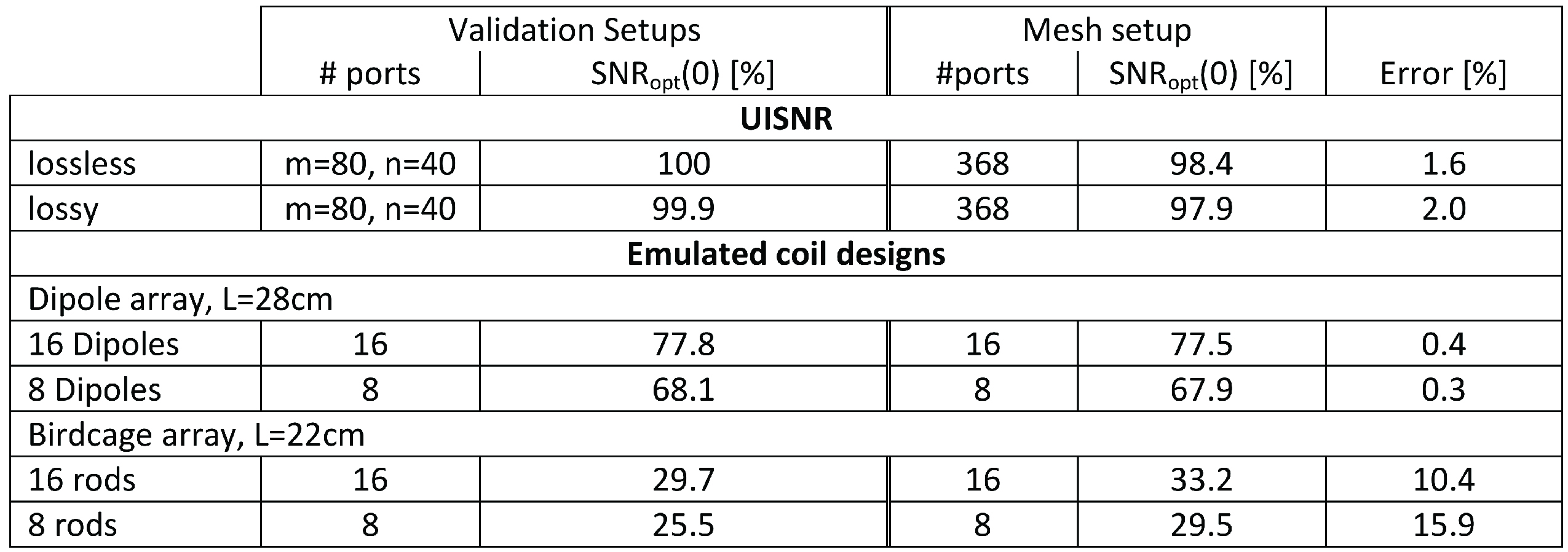
The SNR in the center voxel of the mesh structure compared to validation setup are shown in Table 1. We consider the mesh resolution and length to be sufficient as the lossless mesh setup reaches 98.4% of the lossless UISNR. The validation of the emulated dipole coil arrays are acceptable, however the error in the emulation of the birdcage arrays needs to be further investigated.
The analysis of the optimal currents for the optimal SNR in the center voxel is shown in Fig.3. The optimal currents are in quadrature along the circumference to track the rotation of the spin. The variation of the z- and $$$\phi$$$- directed optimal currents along the z-direction is show in Figs.3a and Fig.3b respectively. The z-directed currents close to z=0 dominate to reach the maximal SNR in the center voxel. The influence of the circumferential currents as well as the z-directed currents that are far away from the center voxel is negligible. We therefore chose the dipole array with a length of 28cm as optimal coil candidates. For completeness the birdcage array with a length of 22cm was also included.
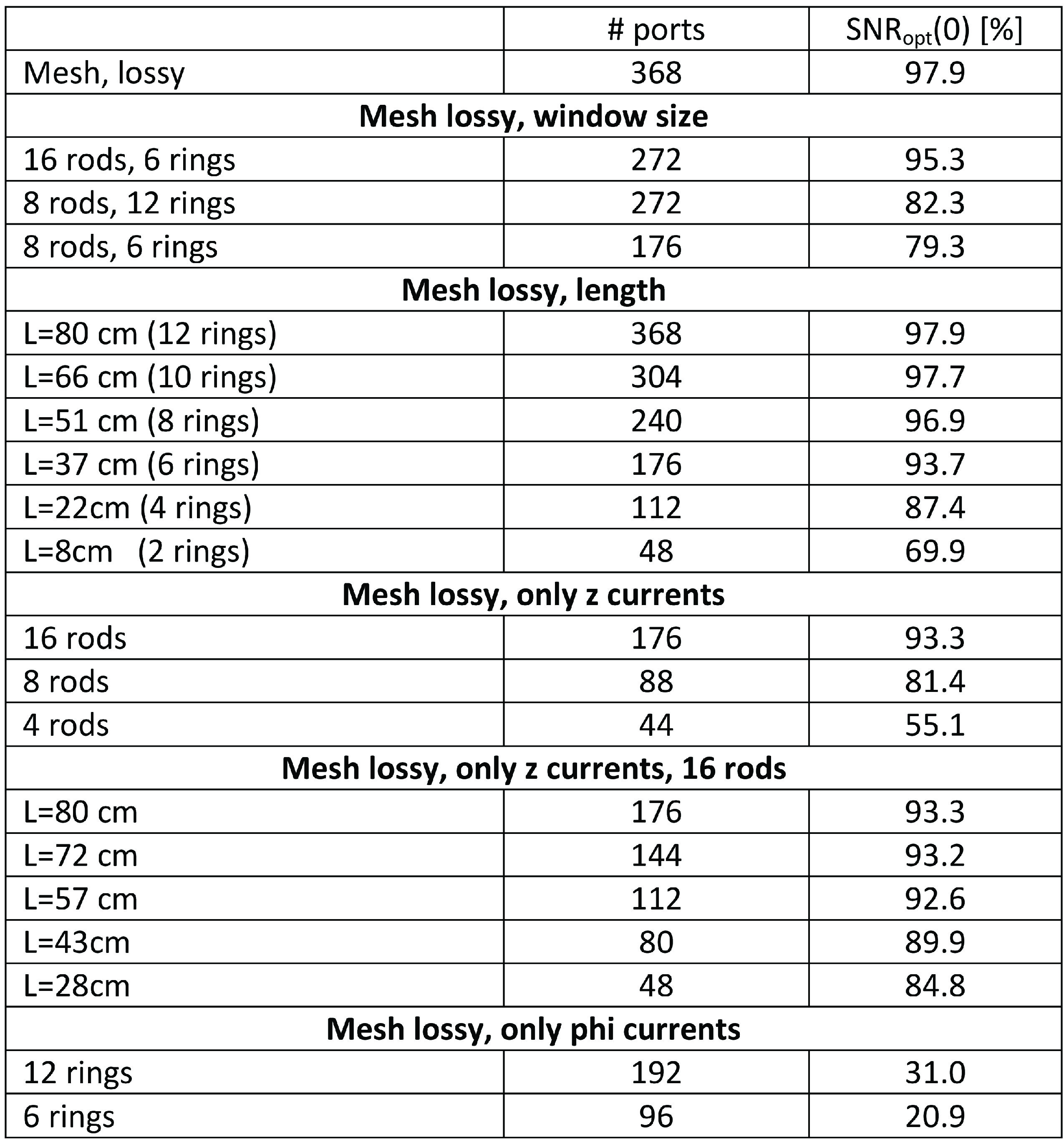
The influence of different setups on the maximal SNR is analyzed in Table 2. As predicted by the optimal current weight analysis, the added benefit of circumferential currents is rather small. The best trade-off between easy construction and high SNR offer designs that allow only z-directed currents that can reach up to 93% of the UISNR. However, as can be seen in Fig.3 the current is phase shifted along the rods, which can be interpreted as a dipole with phase shifters. The construction of such dipoles will be the topic of a future work.
Acknowledgements
No acknowledgement found.References
1. Lattanzi, R., & Sodickson, D. K. (2012). Ideal current patterns yielding optimal signal-to-noise ratio and specific absorption rate in magnetic resonanceimaging: computational methods and physical insights. Magnetic Resonance in Medicine, 68(1), 286–304. http://doi.org/10.1002/mrm.23198
2. Guérin, B., Villena, J. F., Polimeridis, A. G., Adalsteinsson, E., Daniel, L., White, J. K., & Wald, L. L. (2017). The ultimate signal-to-noise ratio in realistic bodymodels. Magnetic Resonance in Medicine, 78(5), 1969–1980. http://doi.org/10.1002/mrm.26564
3. J. Paška, , A. Ruiz, J. Raya, Fast Optimization Method for RF Coil ArrayGeometry in a Post- Processing Step, ISMRM, Intl. Soc. Mag. Reson. Med..p.4401, Paris, France, June 2018.
4. Kozlov, M., & Turner, R. (2009). Fast MRI coil analysis based on 3-D electromagnetic and RF circuit co-simulation. Journal of Magnetic Resonance, 200(1),147–152. http://doi.org/10.1016/j.jmr.2009.06.005
5. C. M. Collins, A. G. Webb, J. Paska, "Electromagnetic Modelling." Magnetic Resonance Technology: Hardware and System Component Design, edited by A.G. Webb, The Royal Society of Chemistry, 2016, pp.331-377
6. Paška, J., Cloos, M. A., & Wiggins, G. C. (2017). A rigid, stand-off hybrid dipole, and birdcage coil array for 7 T body imaging. Magnetic Resonance in Medicine, 00, 1–11. http://doi.org/10.1002/mrm.2704
Figures
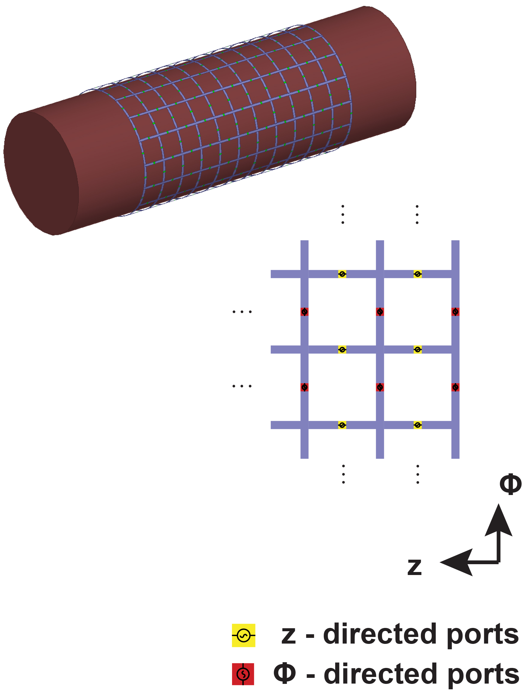
Figure 1: Simulation setup for the mesh structure. The sources can be divided into z- and $$$\phi$$$-directed ports.
The mesh consists of 12 rings, 16 rods and 368 50-Ohm sources, and has a length of 80cm. The mesh is 5mm from the phantom and the conductors have a width of 7mm. The cylindrical surface of the RF-bore as well as the coil conductors were modelled as PEC or as finite conductivity boundary condition, for the lossless and the lossy case respectively. The top and bottom of the RF-bore were terminated with a radiating boundary condition. The numerical domain was discretized in 1.1e6 tetrahedrons. We used second order basis functions.
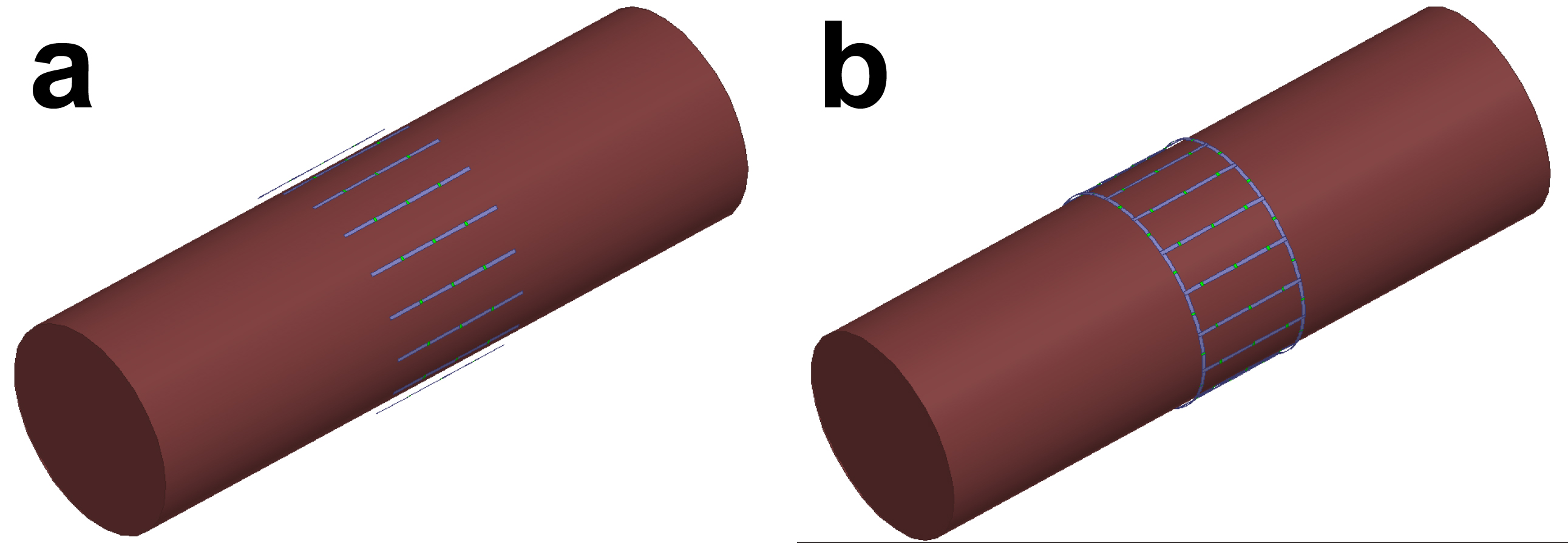
Figure 2: Optimal coil array candidates. a) 16 channel dipole array with a length of 28cm. b) 16 channels birdcage array with a length of 22cm.
The simulation setup is described in Fig1. The conductors of the validation setup trace the conductors of the mesh shown in Fig1. The coil conductors are 5mm from the surface of the phantom and have a width of 7mm. The RF-shield as well as the coil conductors were terminated with a finite conductivity boundary condition with the conductivity 5.8e7S/m. The numerical domain was discretized in 0.42e6 to 1.0e6 tetrahedrons.
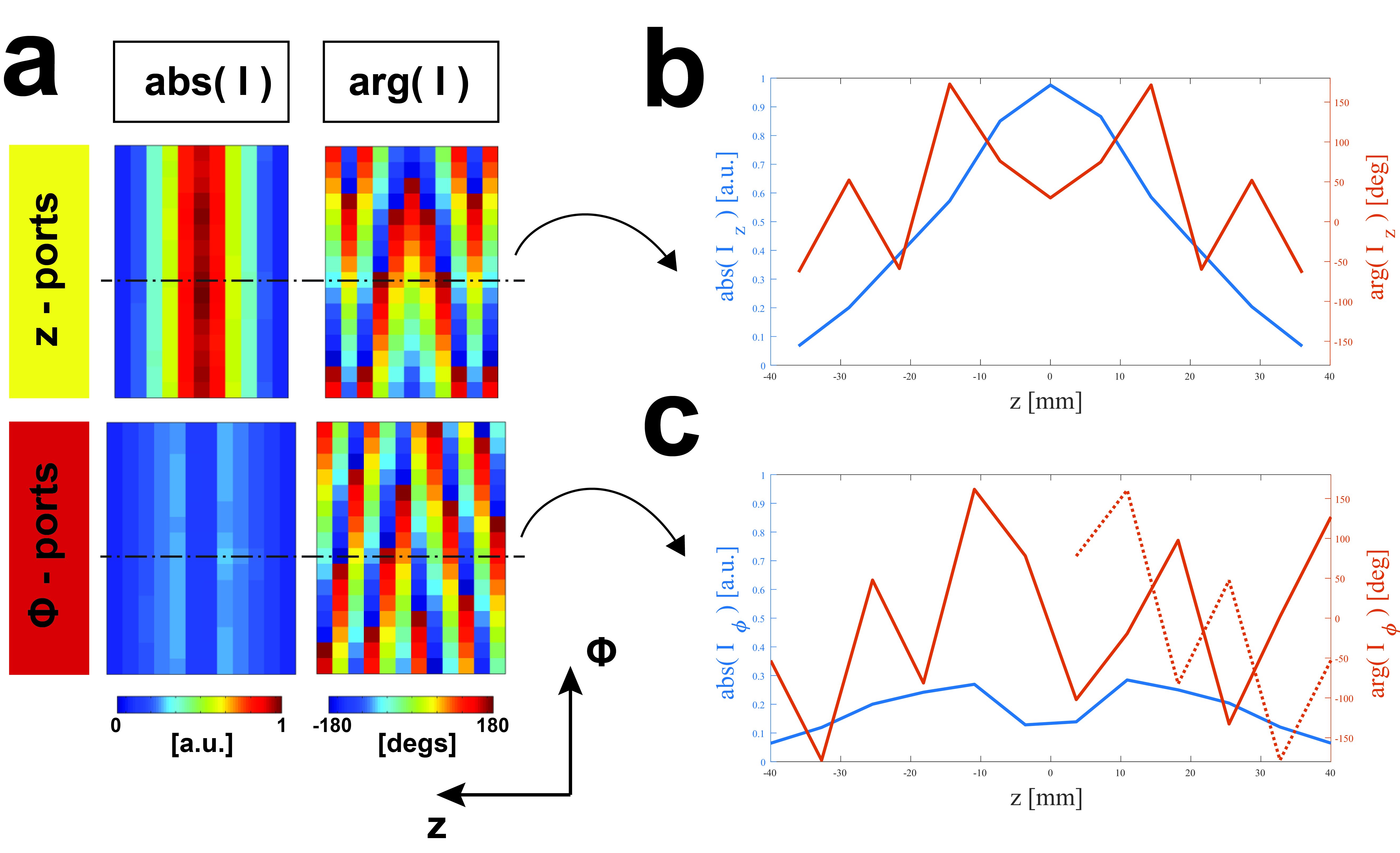
Figure 3: Current weights of the mesh structure for optimal SNR in the center voxel. a) The currents in the z-directed ports and the circumferential ports are shown in the top and bottom row respectively. The left column show the absolute value of the currents in arbitrary units, the right column shows the phase of the currents in degrees. b) Amplitude and phase of the optimal current along the z-direction for the z-directed ports of one rod. c) Amplitude and phase of the optimal current along the z-direction for the phi-directed ports at a given angle.