Introduction

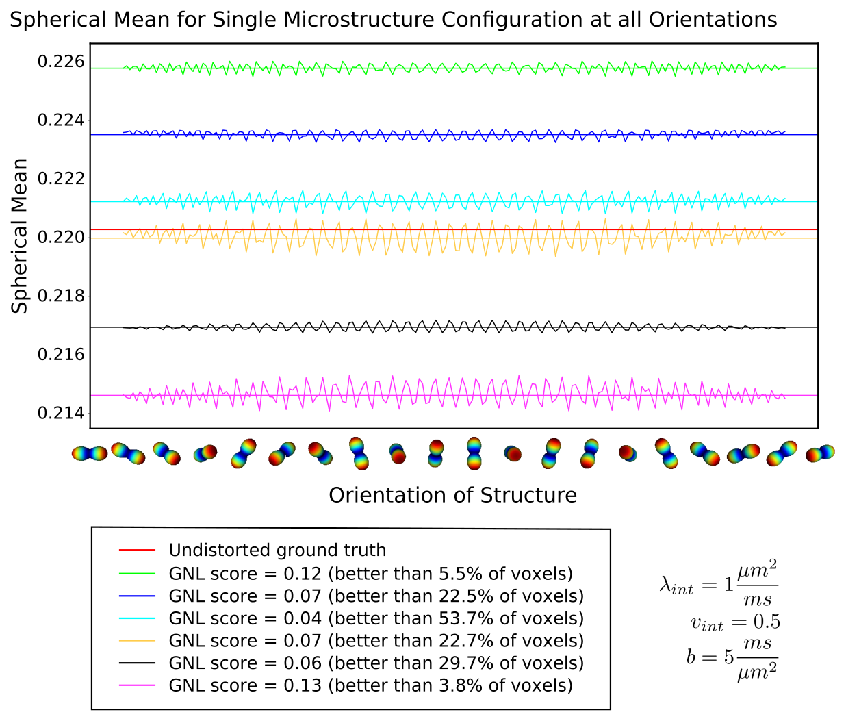
Gradient non-linearity (GNL) in MRI systems induces spatially-varying deviations from the expected gradient direction and intensity¹. These deviations are well described for each gradient system and present a real issue, especially for strong gradient systems². GNL induce geometric distortions and modify the b-values as well as directions of the applied diffusion gradients (DG) at each voxel. Many diffusion models (e.g. DTI³, DKI⁴, MAPMRI⁵) can directly correct for this effect by using the voxelwise GNL adjusted b-values and directions in the model fit. Unfortunately, models depending on shells in b-vector space cannot. One category of such models are the ones which rely on the Spherical Mean (SM) of the diffusion signal. These models fit their parameters on the mean signal from a set of uniformly distributed gradient directions at the same b-value to remove sensitivity to the orientation distribution (OD) from the signal. In the presence on GNL, the SM of the signal is no longer independent of the underlying OD (Figure 3). A natural strategy for correction is to model the signal decay and interpolate to the desired b-shell. One could also interpret the signal as a different b-value that better captures the underlying parameters. In this work, we show the severe effects of GNL on SM and explore options for correction thereof.

Methods

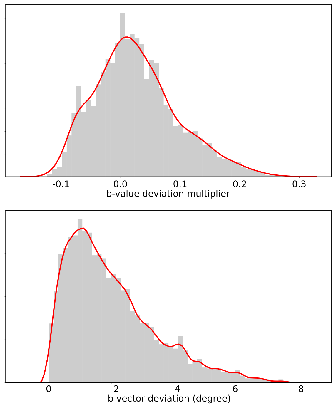
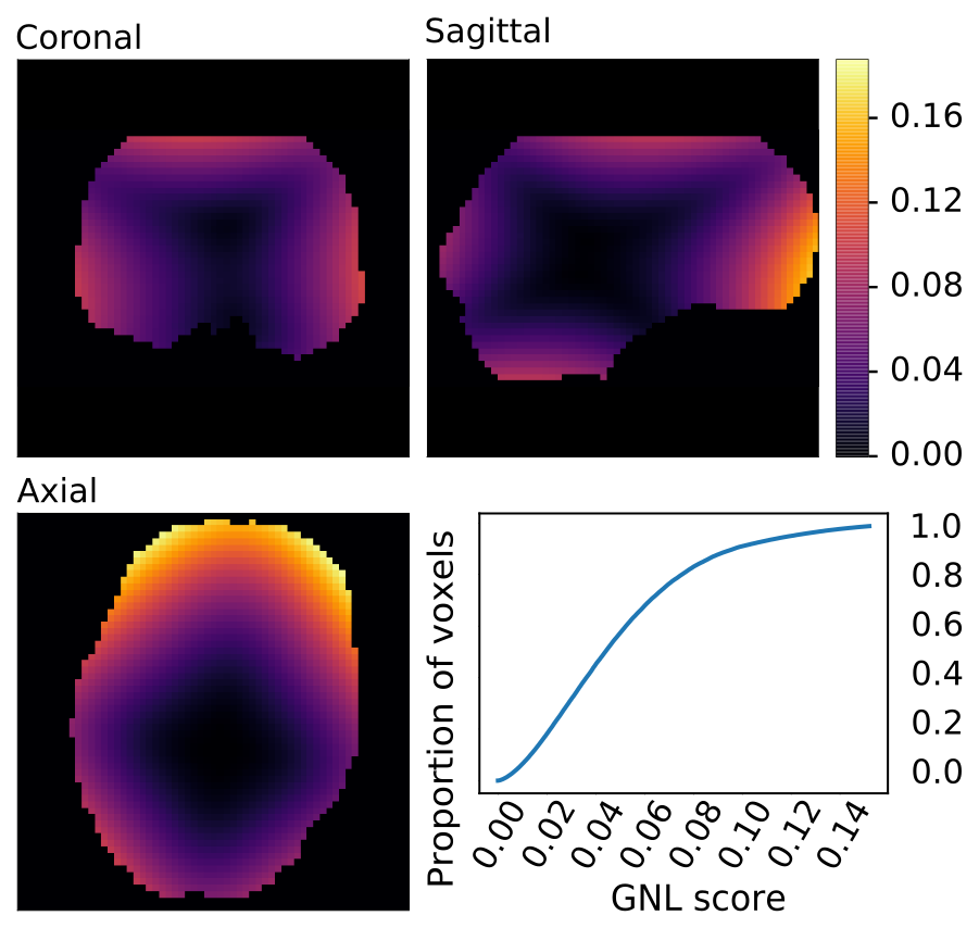
GNL of the MRI system (3T Connectom System, Siemens Healthineers, Erlangen, Germany) were approximated using solid spherical harmonics (order $$$\le$$$ 15) provided by the vendor. For a given dataset, we computed a GNL tensor (GNLT) $$$T$$$ at every voxel $$$i$$$ such that $$$\tilde{g}(i)=T(i)\cdot g$$$ where $$$g$$$ is the planed DG and $$$\tilde{g}$$$ is the spatially varying DG resulting from GNL. Typically, the effects of GNL are more pronounced at the edges of the volume because the severity of GNL depends mainly on the distance to isocenter¹ (figure 2). Figure 1 shows the GNL induced distribution of b-values and direction deviations inside a brain mask of a typical scan on the Connectom system. We explored two modeling strategies for the diffusion signal decay, first-order and second-order. The first-order model fits $$$D_n$$$ at each DG on a single shell such that signal $$$S_n=\exp(-\|\tilde{g}_n\|^2D_n)$$$. The second-order model fits $$$D_n$$$ and $$$K_n$$$ at each DG on a pair of shell such that signal $$$S_n=\exp(-\|\tilde{g}_n\|^2D_n + (\|\tilde{g}_n\|^2D_n)^2K_n/6)$$$. Both models were applied to interpolate a corrected signal for $$$g_n$$$ and spherical averaging was performed. Additionally, we explored a heuristic approach of calculating the mean b-value on the distorted shell and interpreting the signal as an undistorted shell of the mean b-value. To evaluate the accuracy of GNL corrections, we generated a synthetic diffusion signal for multiple microstructural parameters, ODs and GNLTs. A realistic sample of the GNLT space was obtained by clustering the GNLTs inside a representative brain volume. The ODs were generated from mixture of Von-Mises-Fisher distributions for various orientations and concentration parameter $$$k\in [1,16]$$$. We used a microstructure model composed of one stick and one zeppelin compartment modeled by only two free parameters (intra-axonal volume fraction $$$v_{int}$$$ and intra-axonal parallel diffusivity $$$\lambda_{int}$$$). This microstructure model convolved with any OD has a closed form formula for ⁶ We used $$$\lambda_{int}\in [0.5,2.5]\frac{\mu m^2}{ms}$$$ and $$$v_{int}\in [0.1,0.9]$$$ with b-values ranging from 1 to 20 $$$\frac{ms}{\mu m^2}$$$ in the simulations.

Results

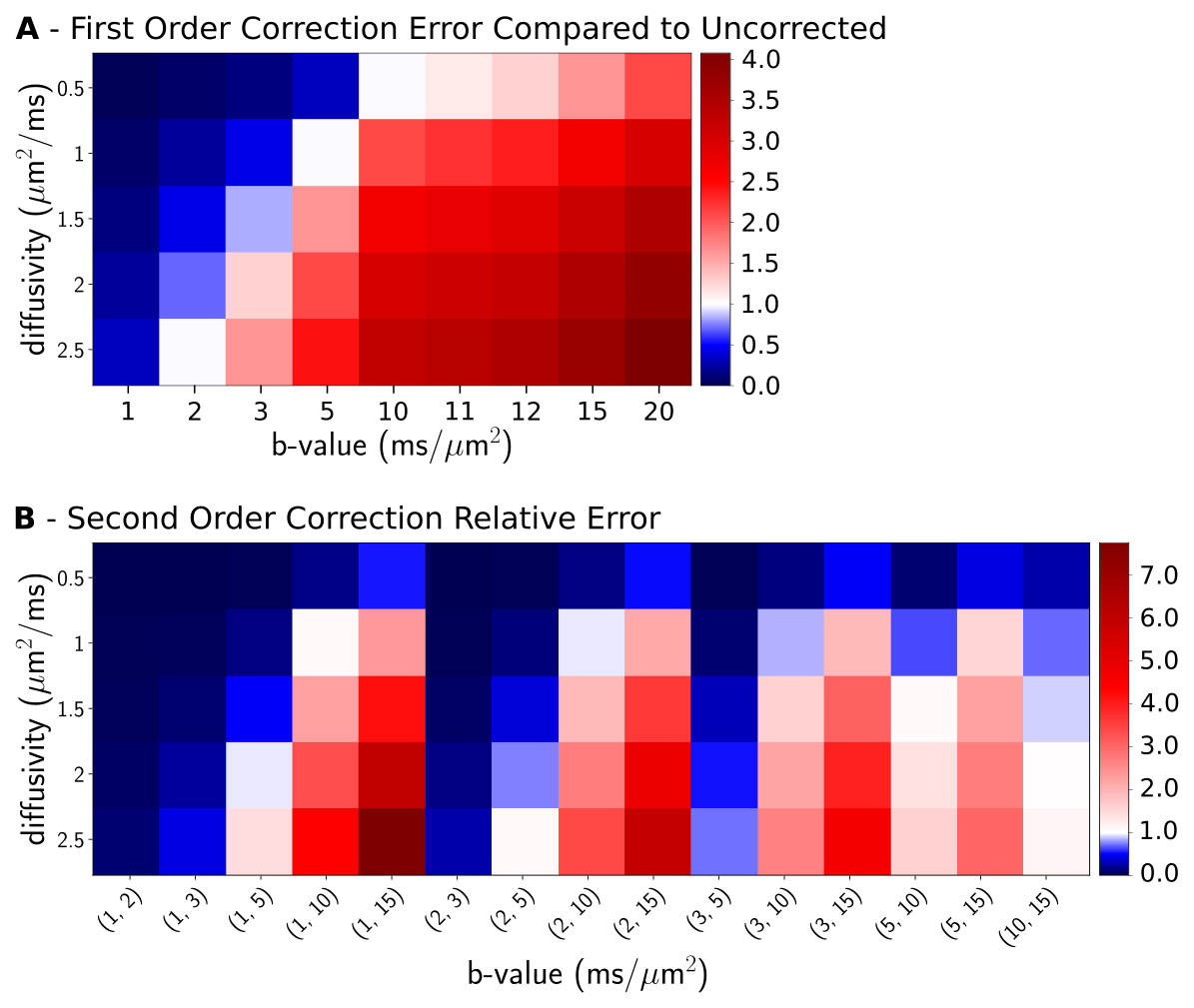
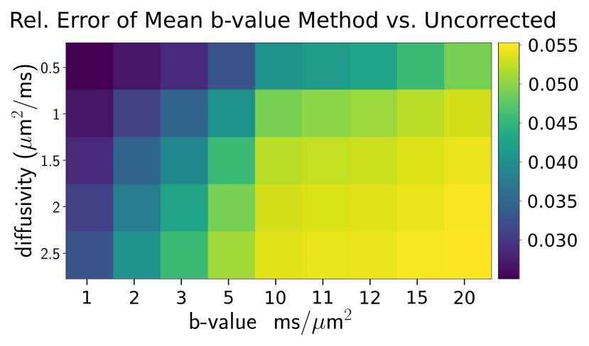
The quality of the first-order and second-order signal approximation is mostly dictated by the product of diffusivity and b-value. Therefore, the first-order recovery (figure 4A) produces spurious results when $$$bD>5$$$. Similarly, the second-order recovery (figure 4B) produces spurious results when using two distant b-values. In practice, it would hard to determine whether or not these models are usable because we do not know the underlying diffusivities. The mean b-value method (figure 5) outperforms the two signal interpolation scheme for all b-values and appear to provide stable error on all configurations. The mean b-value heuristic reduces the GNL bias by 20-fold compared to the uncorrected error.

Discussion

In conclusion, the effects of GNL cannot be ignored when using high strength gradient systems. The anisotropic nature of GNL threatens the separation of the orientation dispersion and diffusion microstructure parameters assumption of SM models. Interpolating the signal to correct the GNL is possible but depends heavily on the underlying diffusion parameters. The simple heuristic of using a shifted b-value and ignoring the orientation dependence reduce the error greatly.

Acknowledgements

MP is supported by a NSERC scholarship (PDF-502732-2017) from Canada.