Introduction

For magnetic resonance spectroscopy (MRS), prevailing methods of metabolite identification and concentration estimation involve fitting algorithms¹ such as LCModel².Especially when processing high spatial resolution 2D/3D-magnetic resonance spectroscopic imaging (MRSI), producing the metabolite concentration maps requires hours or days of computation time, making these methods less usable for end-users such as neuro-radiologists and MR-specialists.³ Machine learning algorithms offer efficient alternative numerical approaches for pattern recognition. Specifically, the deep learning approach with feed-forward multilayered neural network named convolutional neural network (CNN) can recognize accurately particular arrangement of edges, and their position, and assemble patterns into larger aggregate.⁴ These capacities are well suited for complex MR spectra5that are essentially a linear sum of known metabolite signatures plagued by noise and signal residue. This paper compares our CNN approach to a LCModel fitting, on simulated spectra datasets then on in-vivo high-resolution 2D ¹H-FID-MRSI, on their performance for brain metabolite concentration mapping.

Methods

For LCModel, a metabolite basis including high-signal metabolites was created (N-acetylaspartate, N-acetyl aspartylglutamate, creatine, phosphocreatine, phosphorylcholine, glycerophosphorylcholine, myo-inositol, scyllo-inositol, glutamate, glutamine, lactate, beta-glucose and alanine). The supervised learning approach requires large amount of ground truth data to learn from, and real metabolite concentrations are generally unknown in in-vivo conditions. Thus, for CNN training purpose, we produced large amount of artificial data by simulation of ¹H-MRS spectra using well known spin chemical shift and coupling constants of the main metabolites.^3,6 Reference metabolite spectra corresponding to a FID-MRSI sequence at 3T were generated with the GAMMA package⁷ for the metabolites aforementioned.For training, 10⁵ spectra were simulated as the sum of all the metabolite contributions with varying concentrations (Figure 1A & 1B). The resulting metabolites signal is dephased with a random zero and first-order phase and randomly shifted in frequency. Metabolites peaks are randomly broadened. Some random noise as well as a slowly evolving frequency baseline G are added to the signal. To populate the full training dataset, for each spectrum, a set of 30 values are randomly chosen among the required parameters (Figure 1C). Each random parameter were bounded around an acceptable average (e.g., around physiological values for metabolite concentration). CNN training and validation were done using 99%. The 1% remaining was used for the comparison with LCModel. The 104 complex spectral points of one spectrum is the input of the CNN. First a convolutional layer with kernels of the same size as the spectra is applied. The convolutions produce a tensor dataset of features that feed in turn 3 successive hidden layers that ends with the 13 metabolite concentrations of interest as the output. The algorithm then back-propagates to update all the CNN weights. The performance of metabolite concentration estimation was evaluated using the mean error to the known values and the coefficient of determination (R²). We illustrate the use of the two methods on high-resolution 2D-FID MRSI spectra dataset acquired on a human brain.

Results

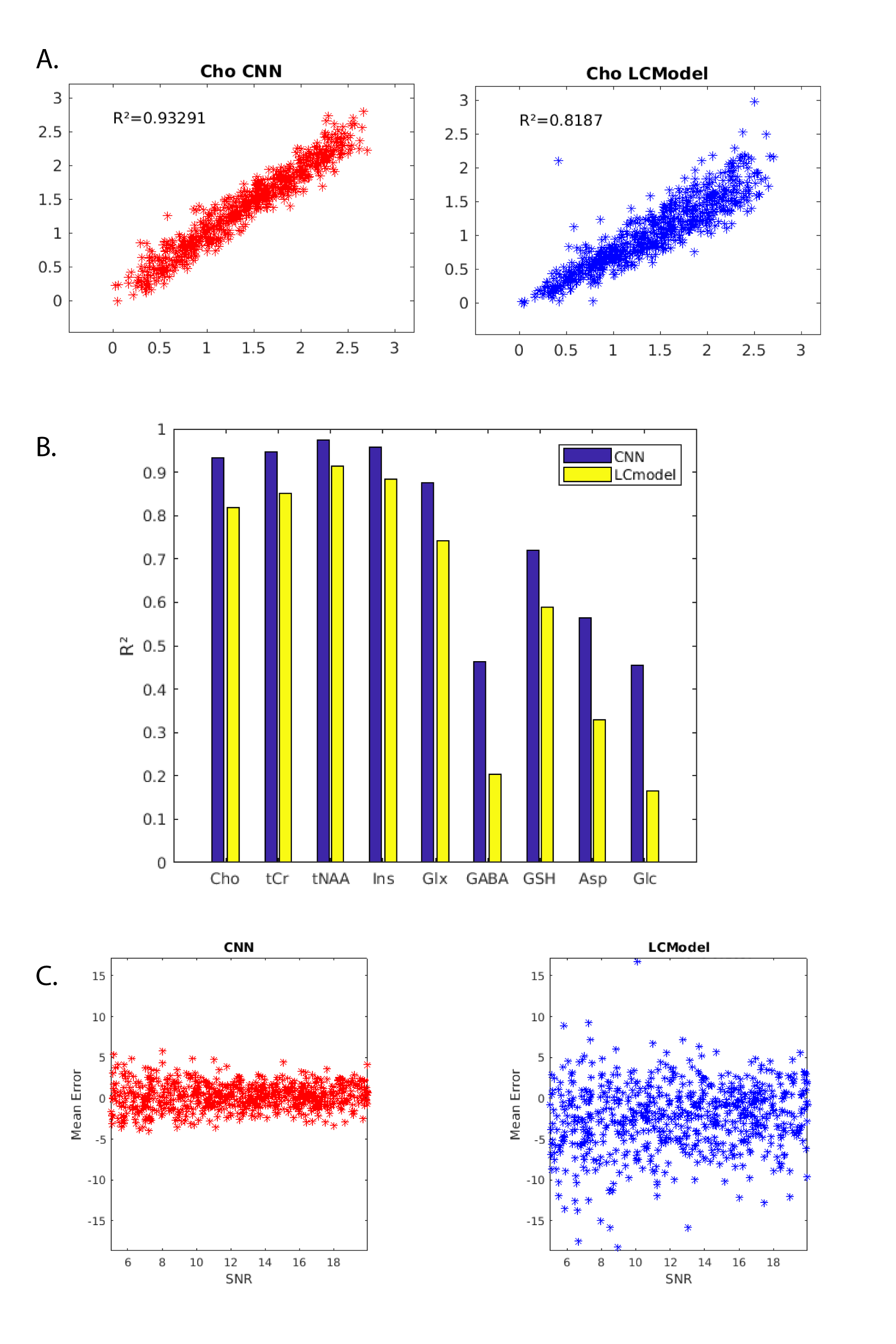
Using a mid-range workstation architecture without high-end GPU, the CNN took approximately 10 minutes to be trained on a full dataset. The trained CNN can quantify a full FID-MRSI data within few seconds while the LCModel can take hours or days. Figure 2 is an LCModel output after fitting with the reference basis aforementioned on a simulated spectrum. For the simulated data, the (Cho) quantification for the test set shows a reduced dispersion of the estimation for the CNN in comparison to LCModel (Figure 3A). The CNN also has a higher R² for all metabolites compared to LCModel (Figure 3B). Finally, the CNN has a lower average mean error as a function of SNR, for all SNR compared to LCModel (figure 3 C). For the in-vivo metabolite mapping, the resulting maps for N-acetylaspartate + N-acetyl aspartylglutamate (figure 4A) and for creatine + phosphocreatine (figure 4B) matches the LCModel results.

Discussion

The performance of the CNN model was better for all metabolites on the simulated dataset. Though CNN or LCModel performance on in-vivo dataset cannot be assessed for certain since true concentrations are unknown, the quantification result by CNN of 2D high-resolution FID-MRSI data of brain was very encouraging. The CNN can achieve comparable results to LCModel even though the data can be plagued by field inhomogeneity, low intensity metabolites signal and macromolecules signal. In addition, the CNN is extremely fast. A trained and optimized CNN can quantify a full FID-MRSI data within seconds, enabling the quasi-direct mapping over reconstructed high-resolution 3D datasets.

Acknowledgements

We thank Dimitri Van Deville for his insights on the convolutional neural network topic.