0470
Learning Perceptual Neural Proximals for Robust MRI Recovery1Electrical Engineering, Stanford University, Stanford, CA, United States, 2Statistics, Stanford University, Stanford, CA, United States, 3Radiology, Stanford University, Stanford, CA, United States
Synopsis
This abstract proposes a framework for robust reconstruction of MR images from highly undersampled measurements. Inspired by proximal gradient descent (PGD) iterations a recurrent neural network is trained to learn a high diagnostic proximal using Wasserstein GANs. For a Knee dataset, the proximal modeled with only two residual blocks shared across 5 iterations not only trains fast but also reveals fine diagnostic details with limited training data. All in all, this study suggests that sharing the proximal weights across iterations regularizes the reconstruction and improves the generalization.
Purpose
Deep learning (DL) has been widely adopted for MRI inverse mapping [1,2,4,6]. Learning a good map however faces severe challenges including: (i) scarcity of high-quality training labels; (ii) high perceptual and diagnostic quality, and (iii) low complexity test and training. We develop a system solving these challenges using as basic architecture the recurrent application of proximal gradient descent (PGD) algorithm. A recurrent ResNet is trained using Wasserstein GANs to learn radiologically plausible proximals. Our key finding with Knee images is that a very light recurrent neural network (RNN) with proximal being a ResNet of 2 residual blocks (RBs) shared across 5 iterations accurately reveals fine diagnostic details of 2D MR images using only a few (<5) training patients under 3 hours of training and 100msec inference.Method
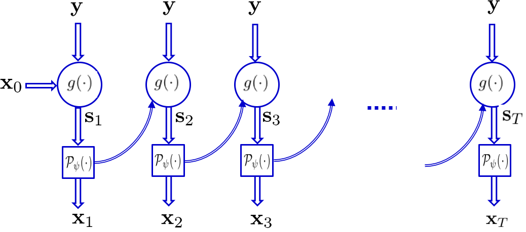
Problem statement. Consider ill-posed MRI problem $$$y=\Phi x_* + v$$$ with $$$\Phi \in \mathbb{C}^{m \times n}$$$ where $$$m \ll n$$$ and $$$v$$$ captures the noise. Suppose the unknown (complex-valued) image $$$x$$$ lies in a manifold $$$\mathcal{M}$$$; no information known about $$$\mathcal{M}$$$ besides (training) samples $$$\mathcal{X}:=\{x_i\}_{i=1}^N$$$ and observations $$$\mathcal{Y}:=\{y_i\}_{i=1}^N$$$. Given a new observation $$$y$$$ the goal is to quickly recover $$$\hat{x} \approx x_*$$$. Our novel idea is inspired by PGD algorithm with a proximal operator $$$\mathcal{P}_{\psi}$$$ [7], where starting from $$$x_0$$$ for step size $$$\alpha$$$ it admits
$$x_{t+1} = \mathcal{P}_{\psi} \Big( x_t + \alpha \Phi^{\mathsf{H}} (y - \Phi x_t) \Big) (1)$$
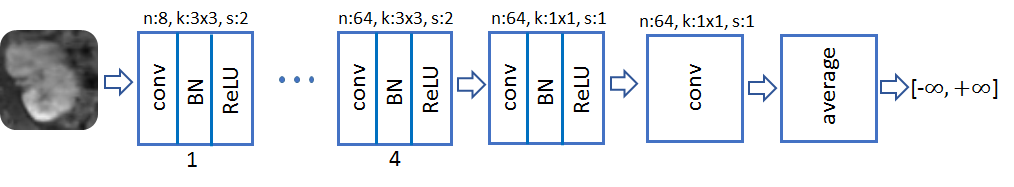
Neural proximal learning. The recursion (1) is envisioned as a state-space model with state variable $$$s_{t+1} = \alpha \Phi^{\mathsf{H}} y + (I - \alpha \Phi^{\mathsf{H}}\Phi )x_{t}$$$ and output $$$x_{t+1} = \mathcal{P}_{\psi}(s_{t+1})$$$ [3]. To model proximal we use a truncated RNN with $$$T$$$ iterations. The measurement y are fed into iterations, which together with the output of the previous iteration form the state variable. The proximal is modeled via ResNet resembling projection onto the manifold of plausible MR images. Output of RNN is fed into a discriminator (D) network and Wasserstein distance metric is adopted with gradient penalty [9] to match the distributions; see [2] for more details.
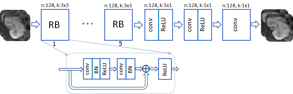
Network architectures. A ResNet with $$$K=2$$$ RBs and $$$T=5$$$ iterations is adopted for G. The real and imaginary image components are considered as two separate channels. Each RB consists of two convolution layers with small 3$$$\times$$$3 kernels and 128 feature maps that are followed by batch normalization (BN) and ReLU activation. D network takes the magnitude of G output after data consistency. It is composed of 8 convolution layers with no BN, and last layer averages out features for classification.
Data. Fully sampled abdominal image volumes are acquired for 350 pediatric patients. Each 3D volume includes 150-220 axial slices of size 256$$$\times$$$128 with voxel resolution 1.07$$$\times$$$1.12 $$$\times$$$2.4mm. Axial slices of 50 patients (9,600 slices) are used for training, and 10 patients (1,920 slices) for testing. All in vivo scans were acquired at the Stanford’s Lucile Packard Children’s Hospital on a 3T MRI scanner [8,10].
Results
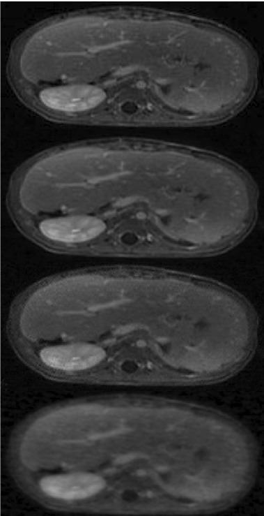
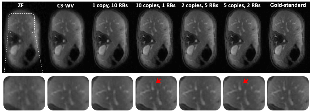
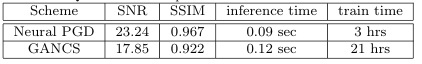
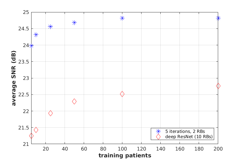
The network is trained to map 5-fold undersampled (variable-density with radial-view ordering) images to fully-sampled ones. For a random test patient, a representative axial slice is shown in Fig. 1 for deep GANCS [1] (10 RBs) and the proposed neural PGD with WGAN proximal. For both schemes 25% WGAN loss and 75% MSE loss is used for training, where neural PGD with WGAN is found more stable with faster convergence (4 times faster). It appears that neural PGD reveals fine details with more natural texture compared with GANCS [1]. It also alleviates the high frequency noise associated with GANCS [1] for large GAN weights (25%). While GAN focuses on perceptual quality, Table 1 indicates neural PGD achieving high SNR/SSIM as well. For train time neural PGD is about 7$$$\times$$$ faster. Looking at outputs of different iterations the early iterations recover low-frequency structural information, while the later layers add high-frequency details. Fig. 2 shows the image recovered for various $$$(K,T)$$$ pairs. Test SNR for different training sample complexities is also plotted in Fig. 6 where one observes that for small training samples (5 patients) there are 3dB performance gains that decreases to 2dB for larger samples (200 patients). All in all, this finding indicates that for MRI recovery it is more beneficial to perform several iterations with shared weights instead of using deep networks for artifact suppression.
Conclusions
This study proposes neural PGD, a RNN trained by Wasserstein GANs to recover radiologicaly plausible images with fine details. It relies on a lightweight training with only for 2 RBs shared 5 iterations demanding a small training sample complexity and achieves high SNR and SSIM, thus a promising solution for MRI recovery problem. Our ongoing research involves more rigorous diagnostic-quality assessment with expert radiologists.Acknowledgements
This research is supported by NIH R01EB009690, NIH R01EB026136, and GE Healthcare.References
[1] Mardani M, Gong E, Cheng JY, Vasanawala SS, Zaharchuk G, Xing L, Pauly JM. Deep Generative Adversarial Neural Networks for Compressive Sensing (GANCS) MRI. IEEE Transactions on Medical Imaging. July 2018.
[2] Mardani M, Sun Q, Vasawanala S, Papyan V, Monajemi H, Pauly J, Donoho D. Neural Proximal Gradient Descent for Compressive Imaging. In Proceeding of Neural Information Processing Systems (NIPS), Montreal, Canada, December 2018.
[3] Michael Lustig, David Donoho, and John M. Pauly. Sparse MRI: The application of compressed sensing for rapid MR imaging. Magnetic Resonance in Medicine, 58(6):1182–1195, December 2007
[4] Jian Sun, Huibin Li, Zongben Xu, et al. Deep ADMM-net for compressive sensing MRI. In Advances in Neural Information Processing Systems, pages 10–18, 2016.
[5] Jo Schlemper, Jose Caballero, Joseph V. Hajnal, Anthony Price, and Daniel Rueckert. A deep cascade of convolutional neural networks for MR image reconstruction. In Proceedings of the 25st Annual Meeting of ISMRM, Honolulu, HI, USA, 2017.
[6] Dongwook Lee, Jaejun Yoo, and Jong Chul Ye. Compressed sensing and parallel MRI using deep residual learning. In Proceedings of the 25st Annual Meeting of ISMRM, Honolulu, HI, USA, 2017.
[7] Neal Parikh, Stephen Boyd, et al. Proximal algorithms. Foundations and TrendsR in Optimization, 1(3):127–239, 2014.
[8] Jonathan I Tamir, Frank Ong, Joseph Y Cheng, Martin Uecker, and Michael Lustig. Generalized Magnetic Resonance Image Reconstruction using The Berkeley Advanced Reconstruction Toolbox. In ISMRM Workshop on Data Sampling and Image Reconstruction, Sedona, 2016.
[9] Gulrajani, Ishaan, Faruk Ahmed, Martin Arjovsky, Vincent Dumoulin, and Aaron C. Courville. "Improved training of wasserstein gans." In Advances in Neural Information Processing Systems, pp. 5767-5777. 2017.
[10] https://github.com/MortezaMardani/NeuralPGD.html.
Figures