0465
Reconstruction of multi-shot diffusion-weighted MRI using unrolled network with U-nets as priors1Department of Electrical Engineering, Stanford University, Stanford, CA, United States, 2Athinoula A. Martinos Center for Biomedical Imaging, Department of Radiology, Massachusetts General Hospital, Harvard Medical School, Boston, MA, United States, 3ByteDance AI Lab, Beijing, China, 4Department of Applied Physics, Stanford University, Stanford, CA, United States, 5Department of Radiology, Stanford University, Stanford, CA, United States, 6Department of Bioengineering, Stanford University, Stanford, CA, United States
Synopsis
In this work, we demonstrated the feasibility of using deep neural networks for rapid multi-shot DWI reconstruction. An unrolled network with six U-nets, which operated in frequency and image domains alternatively, was shown to have the capability to remove aliasing artifacts from shot-to-shot phase
Introduction
Significant aliasing artifacts and signal cancellation may exist in multi-shot diffusion-weighted (DW) MRI due to the motion-induced phase inconsistencies between different shots. A relaxed convex model with a locally low-rank (LLR) constraint has been proposed to reconstruct multi-shot DWIs1, but reconstruction times of 1 minute for a 4-shot image with a matrix size 256-by-256 have limited its application. The purpose of this work was to demonstrate the feasibility of using deep neural networks for rapid multi-shot DWI reconstruction. By using U-nets in both image and frequency domain as trainable priors, and the data consistency constraint, we reduced the required number of iterations from 200 to 6 and achieved almost real-time reconstruction.Methods
Network structure: In shot-LLR, LLR regularization was used to exploit correlations between different shots. In this work, we replace this regularization term with U-nets2 to accelerate the reconstruction process3. By training on large amounts of data, we let the network learn an efficient way to converge to the ground truth. The gradient update based on the data consistency term was kept to help with the convergence and maintain the advantage of model-based methods.
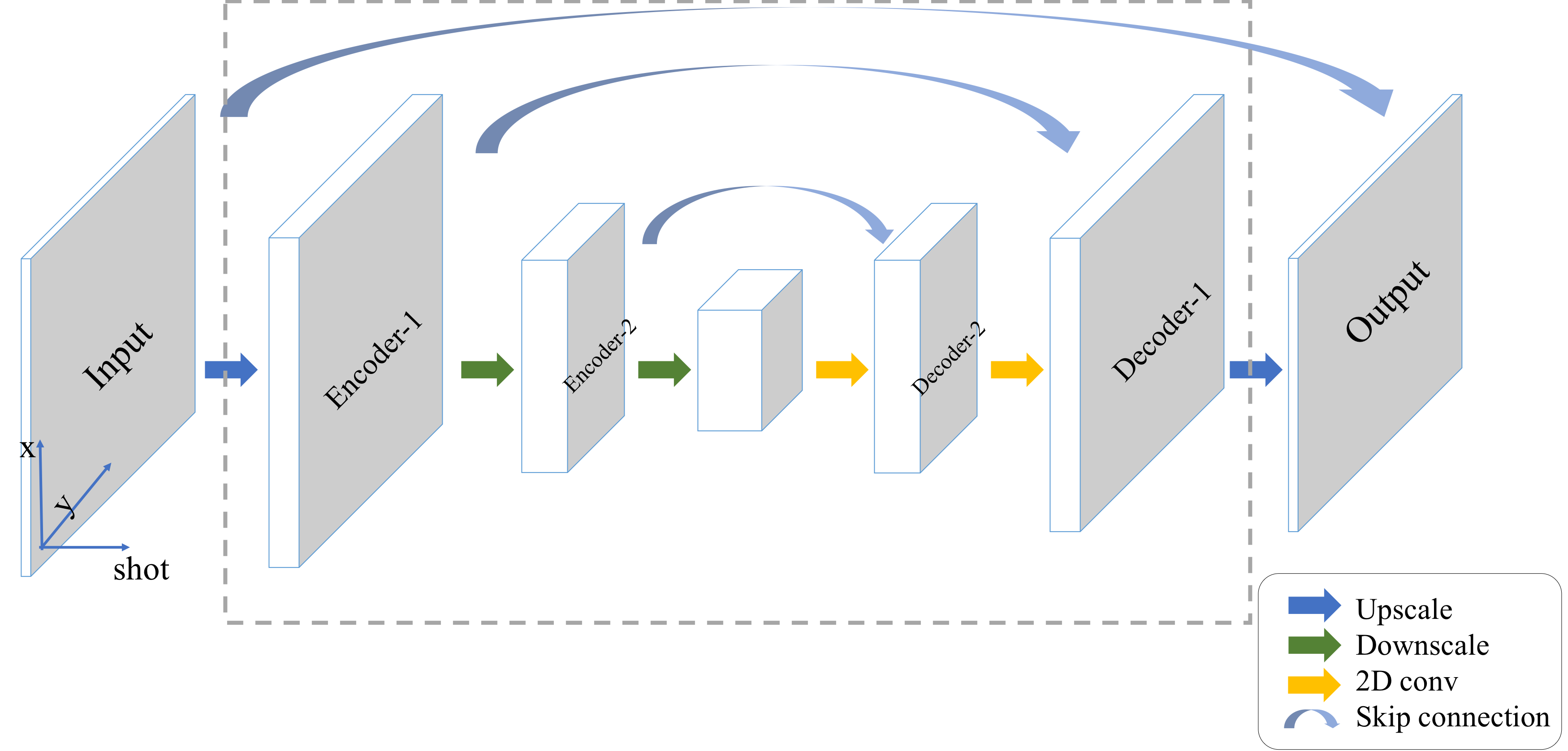
Fig. 1a shows the overall structure of our network: there are 6 iterations in total and a specific U-net in each iteration. Within each iteration, the image is first updated based on the theoretical gradient from the data consistency term, and the updated image is then fed to the neural network to generate images for the next iteration.
Three different architectures are shown in Fig. 1b, and the U-net in each iteration processes data in either frequency domain (K net), image domain (I net) or alternating between frequency and image domain (K-I net)4. Fig. 2 shows the U-net structure, which is the same for each iteration.
Data acquisition: With IRB approval, 1782 axial brain images from seven cases were acquired using a 3T GE MR750 scanner and a 32-channel head receive coil (Nova Medical) with the following parameters: TE/TR = 46/2000 ms, field-of-view (FOV) = 21⨉21 cm2, matrix size = 248⨉244, slice thickness = 3 or 4 mm, number of shots = 4, b-value = 1000 s/mm2, partial Fourier factor = 0.56.
Data formatting: The acquired data were first zero-filled to 256⨉256, and normalized based on the non-diffusion-weighted images. The root-mean-square was used to combine different shots from outputs of the network. 1734 images were used for training and the remaining 48 images were used for testing. Sensitivity maps were calculated from the multi-shot non-diffusion-weighted data using ESPIRiT5 to construct the encoding matrix used in the forward model. Target images were set as the reconstruction results of shot-LLR during training, and L1 difference was used as the loss function.
Results and Discussion
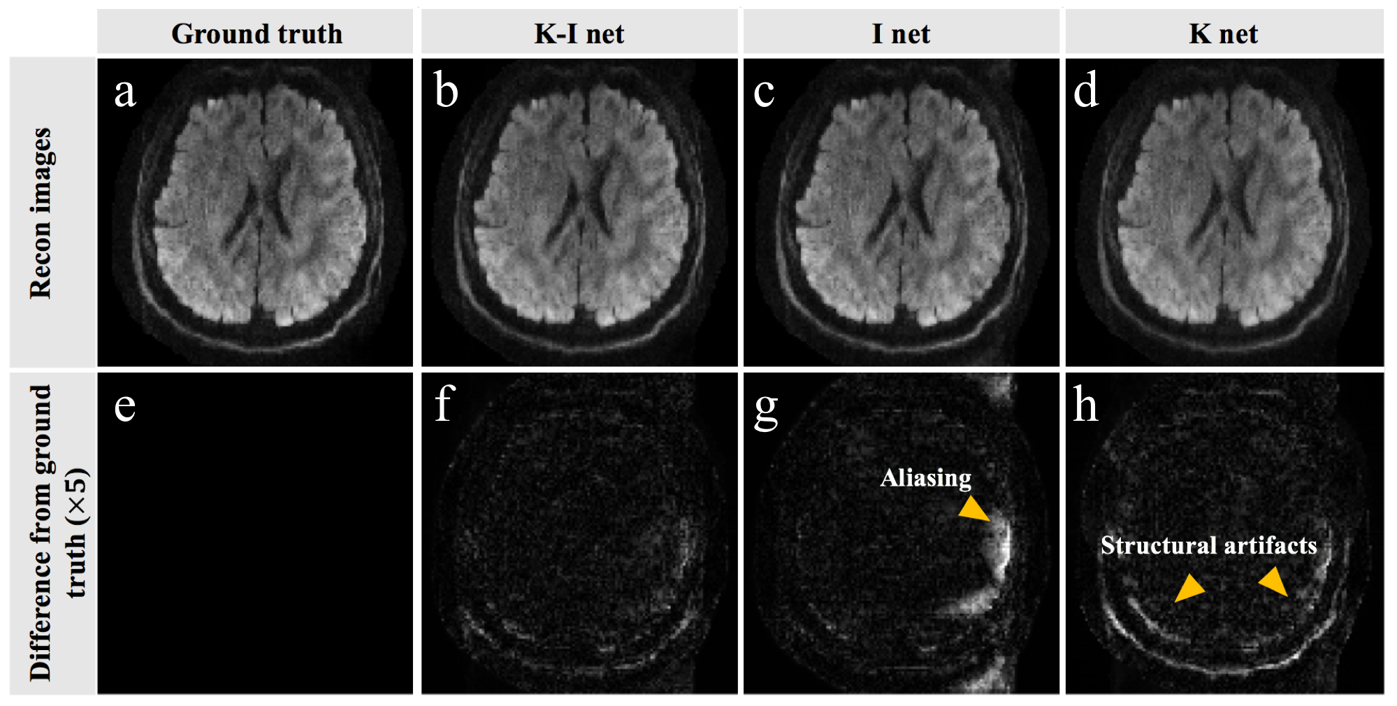
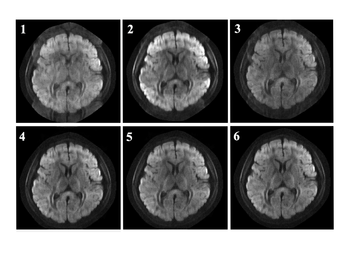
Representative reconstructed images from all three different network architectures are compared in Fig. 3. Fig. 3a is the ground truth from shot-LLR and Fig. 3b-d are from the three networks. Fig. 3c has noticeable aliasing artifacts because the uniform under-sampling in EPI makes it hard for the CNN in image domain to resolve aliasing artifacts. The K net (Fig. 3d) handles aliasing artifacts better. However, learning the intrinsic image property in the frequency domain alone is challenging, which leads to structural artifacts (Fig. 3d). Instead, the reconstructed image from the K-I net (Fig. 3b) is quite close to the ground truth and the difference looks like uniform random noise. Fig. 4 shows the output of each of the six iterations for the K-I net. After first four iterations, almost no residual aliasing artifacts were left, and the following two iterations further refine the image. Networks in different iterations can do different work to achieve different functionalities, which might be another reason why it is more efficient than a fixed constraint.
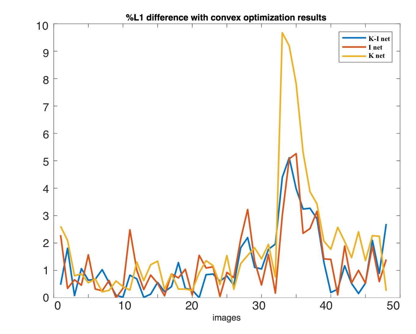
The percentage L1 differences from the ground truth values were plotted in Figure 5. The x-axis of this plot is the image index and the y-axis indicates how different the resulting images are from the targets. The curve for the K-I net in blue is the lowest which has an averaged percentage difference of around 1%.
Conclusion
Acknowledgements
Research support from R01-EB009055, P41-EB015891 and GE Healthcare.References
1. Hu Y, Levine EG, Tian Q, et al. Motion‐robust reconstruction of multishot diffusion‐weighted images without phase estimation through locally low‐rank regularization. Magn. Reson. Med. 2018;00:1–10.
2. Ronneberger, Olaf, Philipp Fischer, and Thomas Brox. "U-net: Convolutional networks for biomedical image segmentation." International Conference on Medical image computing and computer-assisted intervention. Springer, Cham, 2015.
3. Diamond, Steven, et al. "Unrolled Optimization with Deep Priors." arXiv preprint arXiv:1705.08041 (2017).
4. Eo, Taejoon, et al. "KIKI‐net: cross‐domain convolutional neural networks for reconstructing undersampled magnetic resonance images." Magnetic resonance in medicine (2018).
5. Uecker M, Lai P, Murphy MJ, et al. ESPIRiT-an eigenvalue approach to autocalibrating parallel MRI: where SENSE meets GRAPPA. Magn Reson Med. 2014;71:990–1001.
Figures
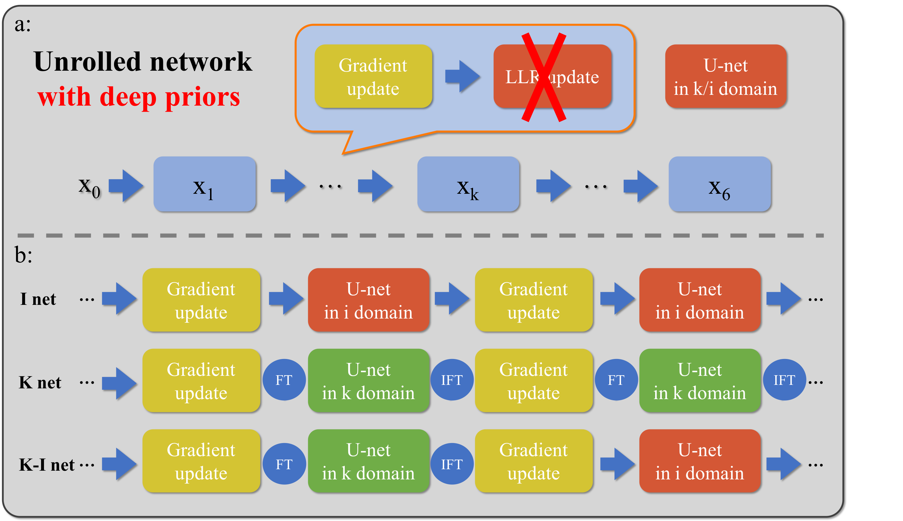
Figure 1a: Schematic diagram of unrolled network with deep priors. There are six iterations and six specific U-nets in total. The output of the previous network is updated based on the data consistency term first before it is given to the next U-net.
b: Three different architectures with U-nets working in image domain (I-net), frequency domain (K-net), or alternating between image and frequency domain (K-I net). There are Fourier transform operator and inverse Fourier transform operator before and after U-net in frequency domain.