0454
3D MR Velocimetry of Very Slow Flows1National Institute of Health, Bethesda, MD, United States, 2University of Florida, Gainesville, FL, United States, 3The Ohio State University, Columbus, OH, United States
Synopsis
Methods are needed to non-invasively measure in vivo very slow flows, which govern many important physiological processes like brain glymphatic flow. In this study, a new stimulated echo-based phase contrast MRI sequence, robust to phase errors induced by gradient hardware, is used to measure 3D flows as slow as 1 μm/s. The method was validated using a controlled pipe flow experiment. In the absence of induced flow, the method revealed unusual natural convection flows in a water filled tube placed in a wide-bore magnet. The method may be applied to measure important slow flows in vivo.
Introduction
Phase-contrast MRI (PC-MRI) velocimetry is routinely used clinically to measure fast flows1, such as blood and cerebrospinal fluid flows, which are on the order of cm/s. However, slow flows govern many important physiological phenomena, such as elevated interstitial fluid flows in tumor2, and glymphatic flows3 in the brain. Currently, few methods exist to measure slow flows non-invasively in vivo within optically opaque tissues. Slow flow encoding with PC-MRI is hampered by diffusion and phase errors introduced by gradient hardware, i.e. eddy currents and mechanical resonances. This study presents a new PC-MRI technique, using stimulated echo (STE) preparation, to overcome these challenges and allows measurement of flows as slow as 1 μm/s.Methods
Measurements were performed on a 330 mm ID, 4.7 T horizontal bore magnet (Oxford Instruments, Abingdon, UK) with an RRI BFG-200/115-S14 gradient set (Resonance Research, Billerica, MA) using an Agilent VNMRS imaging console running VnmrJ3.1A software (Agilent Technologies, Santa Clara, CA). RF was transmitted and received using 38 mm ID volume quadrature birdcage coil (Varian, Inc, Palo Alto, CA).
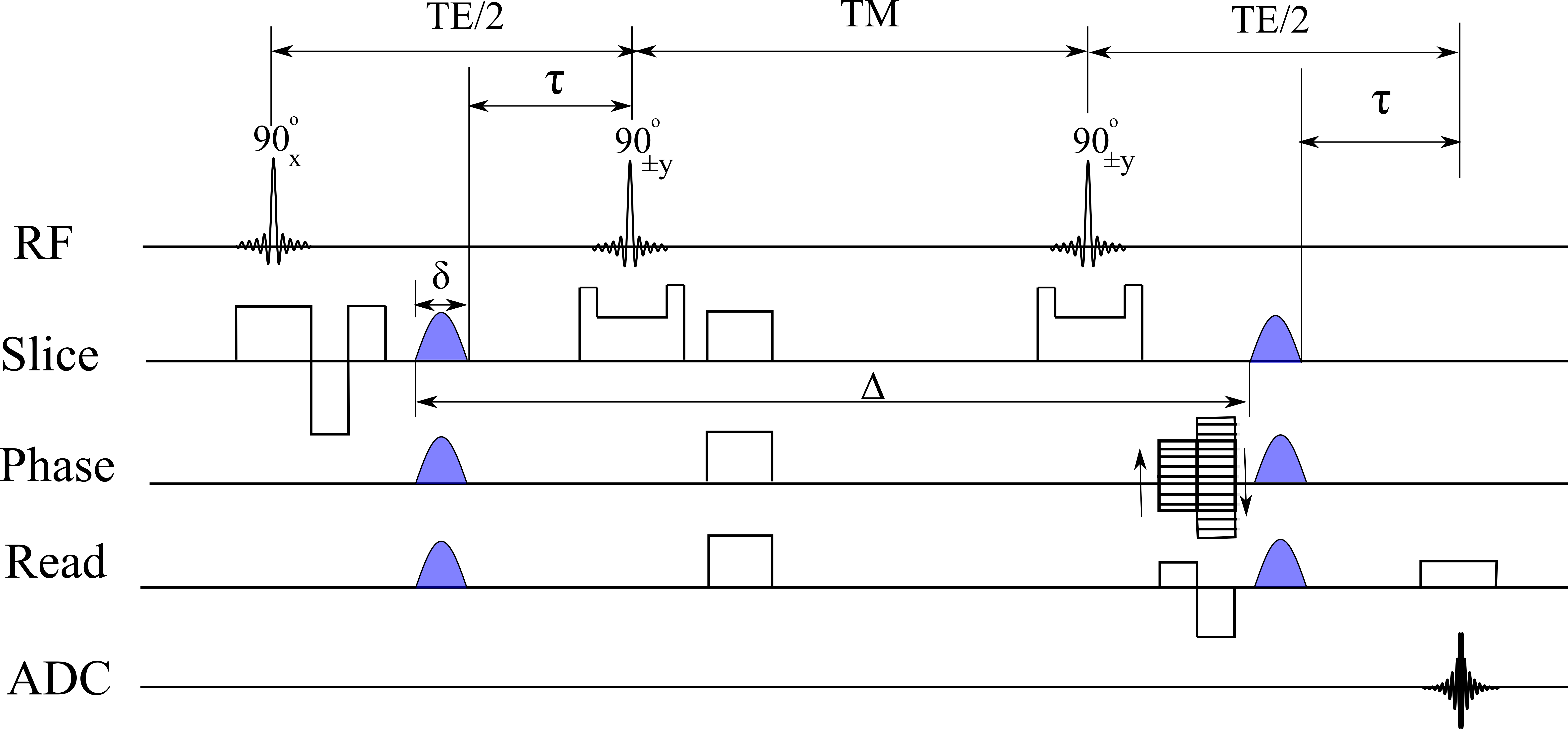
The new PC-MRI pulse sequence is shown in Figure 1. Four acquisitions were performed per voxel to measure the 3D flow with flow gradients simultaneously applied on all three axes with different polarities set based on the Hadamard encoding4. The velocities were extracted by complex dividing the MR images appropriately4. Since the diffusion weighting (b-value) has quadratic dependence on the displacement wave vector, q (proportional to gradient area), and the velocity encoding is linearly dependent on q, the effect of diffusion is reduced by using a small q while the concomitant loss of velocity sensitivity was partly compensated by using a long mixing time afforded by STE. Flow weighting factor, venc, as small as 40 μm/s was achieved using this method. Static spin phase due to eddy current magnetic fields generated from the flow-encoding gradient pulses was refocused at the echo time by equalizing the time interval, τ
The method was validated using controlled pipe flow through silicone tubes filled with water connected to a syringe pump. A static gel phantom was placed alongside the tube to monitor flow-independent phase errors. Flow measurements were performed at two different flow rates (Q = 2, 10 μL/min). In addition, natural convection flow measurement was performed on a water filled 15 mL cylindrical tube placed in the magnet bore alongside a tube filled with 0.6% (w/v) hydrogel.
Flow imaging data for
pipe flow was acquired for two 8 mm thick axial slices in the center straight
section of the tubes with FOV = 32 mm × 32 mm, matrix size = 96 × 96, TR/TE = 4500/28 ms, NEX = 2, half-sine shaped flow encoding gradient pulses with δ = 0.5 ms of strength = 120 mT/m and pulse separation, Δ = 2000 ms, resulting in a venc ≈ 38 μm/s. Flow imaging data for the natural convection sample was acquired for a single 8 mm thick axial slice with a FOV = 32 mm × 16 mm, matrix size = 128 × 64, NEX = 2, TR/TE = 3000/28 ms, and half-sine shaped flow encoding gradient pulses with δ = 0.5 ms of strength = 120 mT/m and pulse separation, Δ = 500 ms (venc ≈ 150 μm/s).
Results and Discussion
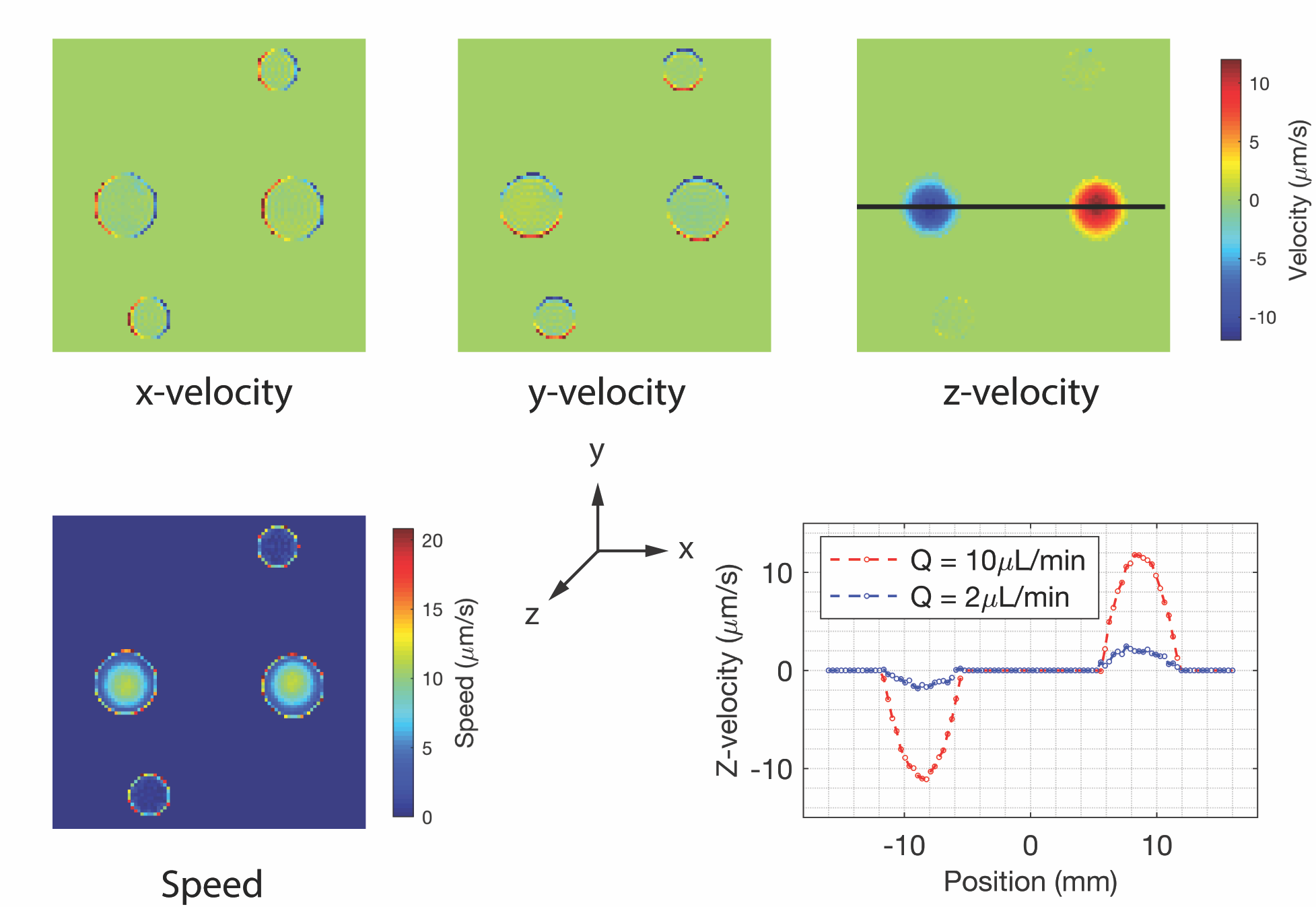
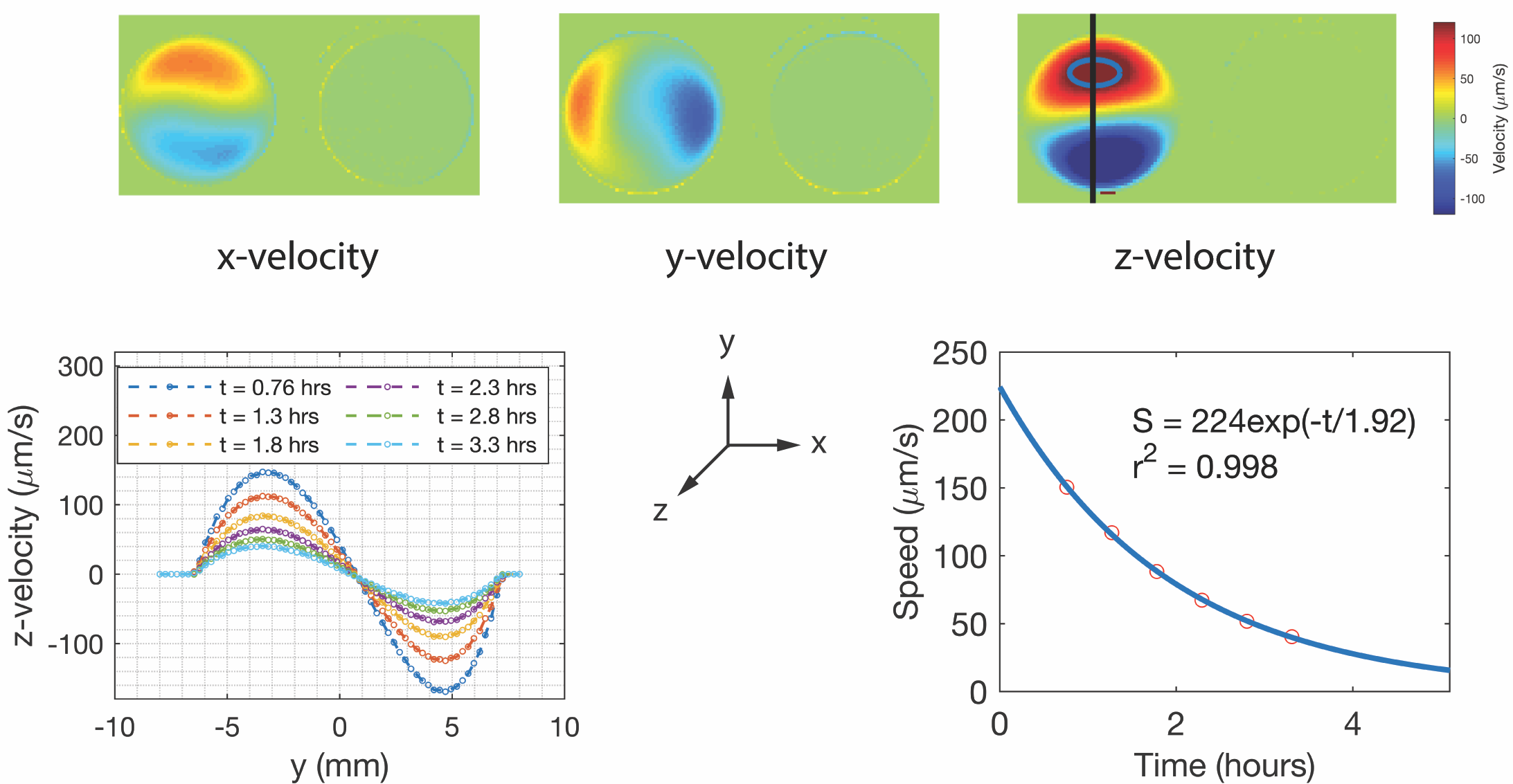
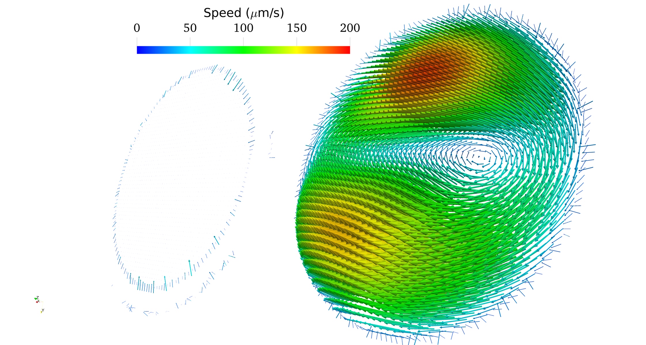
A pipe flow 3D velocity map is shown in Figure 2. The results show the expected parabolic velocity profile in the axial direction with peak velocities close to 2,10 μm/s, as expected for Q = 2, 10 μL/min flows. Phase errors in static phantom albeit small (0.45 to 4.45 μm/s across the 32 mm readout FOV) were visible in the readout dimension due to gradient echo shifts within the generated STE. These were removed post-processing by fitting a linear phase variation across the FOV. Natural convection measurements show a complex 3D vortex primarily in the axial direction (Figure 3 and 4), which was absent in the gel filled tube. This flow may be due to temperature gradients present along the length of the bore caused by inhomogeneous heat transfer to the sample or heating of the gradient coil. This convection flow decreases exponentially with a time constant of approximately 2 hours (Figure 3). Such flows in non-variable temperature (VT) probes in horizontal bore magnets has not been reported previously. This method may allow the study of very slow flows in tissue, such as convection flow, interstitial flows in tumors, and perhaps glymphatic flow.Acknowledgements
A portion of this work was performed in the Advanced MRI/S (AMRIS) Facility at the McKnight Brain Institute of the University of Florida, which is part of the National High Magnetic Field Laboratory (supported by National Science Foundation Cooperative Agreement DMR-1157490, the State of Florida, and the U.S. Department of Energy). In addition, this work is supported in part by the NIH/NCATS Clinical and Translational Science Award UL1 TR000064. We would like to thank Dr. Alan Rath from Agilent Technologies for advice on pulse programming, and Dr. Huadong Zeng and Kelly Jenkins from the AMRIS Facility for assisting with experimental setup.References
1.Mase, M. et al. Quantitative Analysis of CSF Flow Dynamics using MRI in Normal Pressure Hydrocephalus. in Intracranial Pressure and Neuromonitoring in Brain Injury 350–353 (Springer Vienna, 1998).
2. Munson, J. M. & Shieh, A. C. Interstitial fluid flow in cancer: implications for disease progression and treatment. Cancer Manag. Res. 6, 317 (2014).
3. Asgari, M., de Zélicourt, D. & Kurtcuoglu, V. Glymphatic solute transport does not require bulk flow. Sci. Rep. 6, 38635 (2016).
4. Haacke, E. M., Brown, R. W., Thompson, M. R. & Venkatesan, R. Magnetic Resonance Imaging: Physical Principles and Sequence Design. (Wiley, 1999).
Figures