0453
Reynolds Stress Tensor Quantification using a Flow-MRF Approach1German Cancer Research Center (DKFZ), Heidelberg, Germany, 2Physikalisch-Technische Bundesanstalt (PTB), Braunschweig and Berlin, Germany
Synopsis
This work demonstrates the feasibility to quantify simultaneously the Reynolds stress tensor and velocities using a Flow-MRF based approach in conditions of turbulent flow. This is achieved by measuring spatially undersampled time-series with pseudo-randomly varying velocity encoding moments, based on the MR Fingerprinting framework.
Introduction
Flow-MR Fingerprinting (Flow-MRF) is a recently presented technique1,2 that allows simultaneous quantification of time-resolved velocities and relaxometric parameters of static tissue, based on the MRF framework3. The velocity quantification is performed by measuring spatially undersampled time series with pseudo-randomly varying velocity encoding moments. This allows the use of high velocity encoding moments (m1) while maintaining a large dynamic range of quantifiable velocities at shorter measurement times than those of standard single-venc sequences1. The characterization of turbulent flow conditions with MRI has been demonstrated by measuring the velocity-encoding-related signal loss4-6 , and, recently, the quantification of the Reynolds stress tensor (RST) was shown using this approach7. The RST quantification requires at least 6 non-orthogonal multidirectional velocity encodings and a velocity compensated measurement, leading to long acquisition times using conventional acquisition strategies. In contrast, the inherent use of many non-orthogonal velocity encoding directions in Flow-MRF makes this technique highly attractive for the quantification of RST in turbulent flow conditions. This work investigates the feasibility of using Flow-MRF-like acquisitions strategies for the quantification of turbulent conditions.
Theory
The Reynolds stress tensor $$$\tau$$$ can be obtained by solving the following equation based on N velocity-encoded measurements.
$$$\begin{bmatrix}k_{x,1}^2&k_{y,1}^2&k_{z,1}^2&k_{x,1}k_{y,1}&k_{x,1}k_{z,1}&k_{y,1}k_{z,1}\\{\vdots}&\vdots&\vdots&\vdots&\vdots&\vdots\\k_{x,N}^2&k_{y,N}^2&k_{z,N}^2&k_{x,N}k_{y,N}&k_{x,N}k_{z,N}&k_{y,N}k_{z,N}\end{bmatrix}\begin{bmatrix}\tau_{xx}\\\tau_{yy}\\\tau_{zz}\\\tau_{xy}\\\tau_{xz}\\\tau_{yz}\end{bmatrix}=\begin{bmatrix}-2ln\left(\mid\frac{S({\bf{k}}_1)}{S(0)}\mid\right)\\{\vdots}\\-2ln\left(\mid\frac{S({\bf{k}}_N)}{S(0)}\mid\right)\end{bmatrix}$$$
with
$$${\bf{k}}_n=\gamma[m_{1,x,n},m_{1,y,n},m_{1,y,n}]\quad{n}\in{\{1,\dots,N\}}.$$$
Here, $$$\gamma$$$ is the gyromagnetic
ratio, S(kn) the measured signal for velocity encoding kn and S(0) the signal of a velocity-compensated measurement. For Flow-MRF
N equals approximately 50 and depends
on the volunteer’s heart rate, while S(0)
is unknown and is to be estimated alongside the stress tensor.
Methods
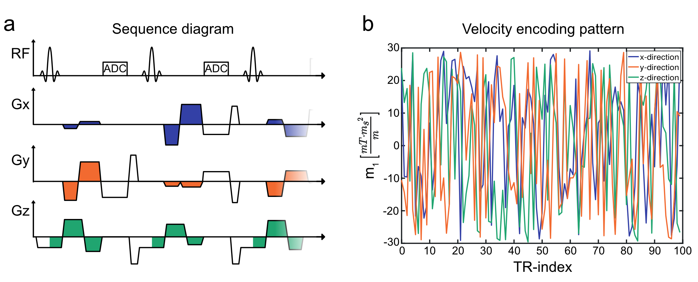
The sequence diagram of the radial Flow-MRF sequence is shown in Fig.2 along with a portion of the velocity encoding pattern. The pattern consists of a white noise distribution with a maximum $$$\Delta{m_1}$$$ of 60 corresponding to a 20cm/s encoding velocity (venc). Unlike the previously shown implementations of Flow-MRF1,2,8, no inversion preparation was used and the flip angle (FA) was fixed for all TRs, preventing T1 and T2 quantification. Preliminary investigations revealed that variable FAs would result in complex dependencies of S(0) on the FA pattern, the inflow behavior and the relaxation times of the fluid. In the case of a fixed FA, signal magnitude is a function only of S(0) and RST, while the signal phase uniquely encodes the mean velocity of a voxel.
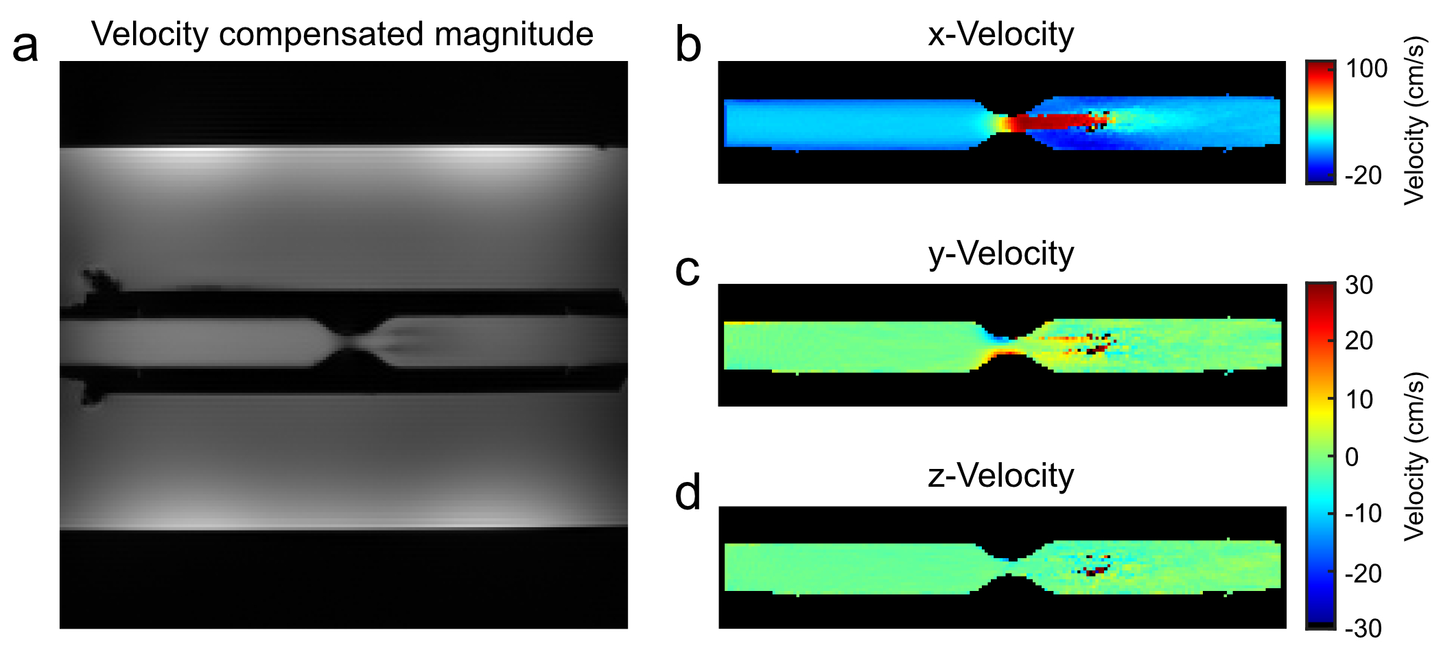
The quantification of RST was performed in a coronal slice through a stenosis phantom as displayed in Fig.1a. In this phantom the stenosis reduces the diameter of the lumen from 15mm to 5mm, resulting in an approximately 9-fold velocity increase. The velocity jet creates turbulent flow regimes at its edges as shown in Fig.1. The turbulence causes the velocity distribution (assumed Gaussian2) to strongly widen (Fig.1b), which results in decreased signal magnitudes due to intravoxel dephasing (Fig.1d). This widening of the velocity distribution is not captured by normal velocity quantification as only a mean velocity is assigned to each voxel.
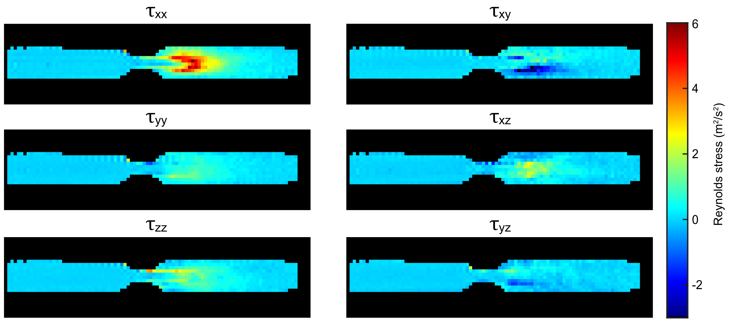
All measurements were performed using a 28-channel knee coil (Quality Electrodynamics, USA) at a 7T system (Magnetom 7T, Siemens, Germany). The Flow-MRF sequence was acquired with 30 radial projections per frame in 3min 59s with a spatio-temporal resolution of 0.8×0.8×5mm3/39.2ms. To increase the signal for the RST maps, the reconstructed in-plane voxel size was doubled (1.6×1.6×5mm3) during reconstruction. A 3D phase-contrast GRE with an ICOSA6 velocity encoding pattern, venc of 0.5m/s and resolution of 1.5×1.5×1.5mm3 as presented by Haraldsson et al.7 was measured as a reference for the RST quantification.
Results
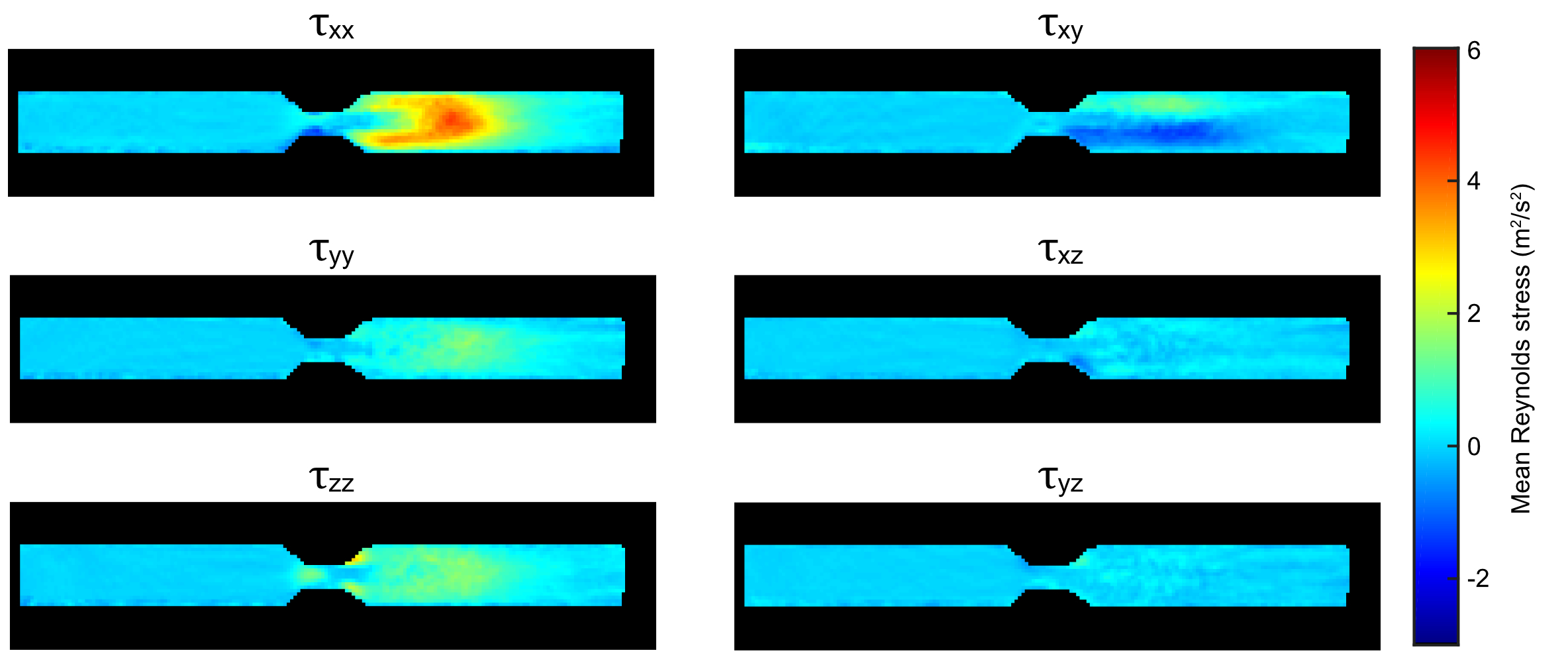
Figure 3 shows a cardiac phase from the velocity mapping results based on Flow-MRF. The mean velocity upstream of the stenosis is 11.9cm/s, increasing to 103.9cm/s within the stenosis, which matches the expected 9-fold velocity increase. The velocity quantification fails in a few pixels at the end of the velocity jet due to strong signal dephasing. This is supported by the $$$\tau_{xx}$$$ component in Fig.4a showing the highest degree of signal dephasing in such locations. The comparison of the stress components between Flow-MRF and the reference shows qualitatively a good agreement in turbulence shape and magnitude even though the peak stress is 14% lower for Flow-MRF (see Fig.4&5).
Discussion
In this work, we demonstrate the feasibility of simultaneously quantifying RST and velocities using a Flow-MRF-based approach. Both the conventional and the Flow-MRF sequence provide similar RST components despite the dissimilar spatial resolution. The larger slice thickness of the Flow-MRF sequence might have caused the lower peak stress and low stress in the $$$\tau_{xz}\,\,$$$and$$$\,\,\tau_{yz}$$$ components. The area of turbulence appears larger in Flow-MRF, which might be linked to a greater sensitivity to turbulence due to the higher velocity encoding moments. While higher moments also reduce the signal for the velocity quantification, this balance can be optimized through the choice of velocity encoding patterns in Flow-MRF.Acknowledgements
No acknowledgement found.References
- Flassbeck S. et al. Flow MR Fingerprinting (in press). DOI: 10.1002/mrm.27588
- Flassbeck S. et al. Quantification of Flow by Magnetic Resonance Fingerprinting. In Proc. 25th ISMRM, 2017
- Ma D. et al. Magnetic Resonance Fingerprinting. Nature, 2013
- Dyverfeldt P. et al. Quantification of Intravoxel Velocity Standard Deviation and Turbulence Intensity by Generalizing Phase-Contrast MRI. MRM, 2006
- Dyverfeldt P. et al. Assessment of Fluctuating Velocities in Disturbed Cardiovascular Blood Flow: In Vivo Feasibility of Generalized Phase-Contrast MRI. JMRI, 2008
- Dyverfeldt P. et al. On MRI turbulence quantification. MRI, 2009
- Haraldsson H. et al. Assessment of Reynolds Stress Components and Turbulent Pressure Loss Using 4D Flow MRI With Extended Motion Encoding. MRM, 2018
- Flassbeck
et al. Flow-MRF: a novel way of quantifying blood velocities in combination
with tissue relaxation parameters. In Proc. 30th SMRA, 2018
Figures
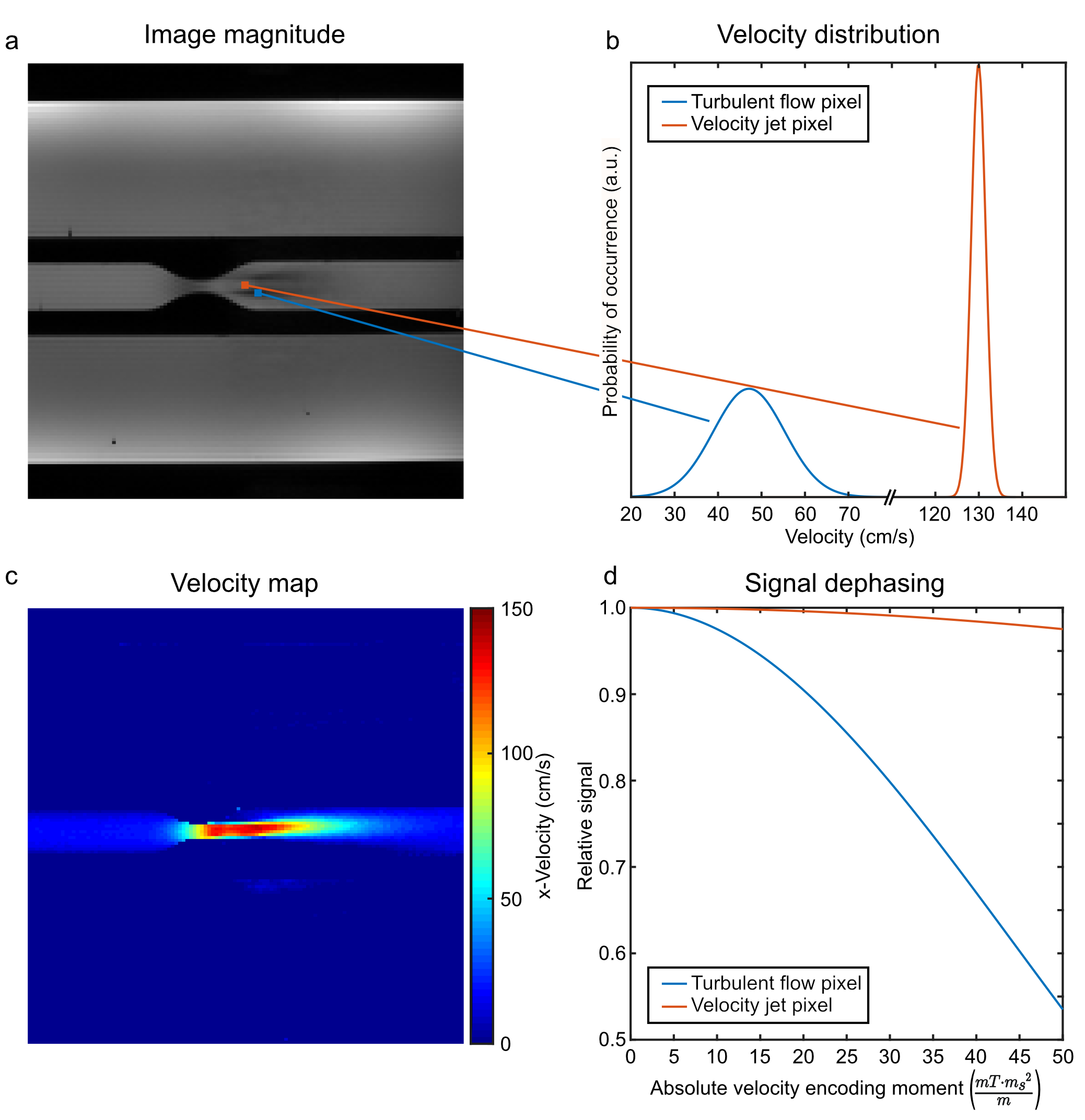
Figure 1: Schematic overview of signal dephasing due to turbulent flow in a stenosis phantom. (a) shows the magnitude of a standard velocity-encoded 2D-Cine; the signal drop after the stenosis is caused by turbulent dephasing. (b) schematically indicates the intravoxel velocity distribution within the laminar flow of the jet and the turbulent flow adjacent to the velocity jet. The velocity map corresponding to the measurement of (a) is displayed in (c). The relative signal loss as a function of the velocity encoding moment is plotted in (d) for the two distributions shown in (b).