0447
Dwell Time Compensation of the Gradient System Transfer Function (GSTF): Field Camera versus Phantom-based Measurement1Department of Diagnostic and Interventional Radiology, University Hospital Würzburg, Würzburg, Germany, 2Cardiovascular Branch, National Heart, Lung, and Blood Institute, National Institutes of Health, Bethesda, MD, United States
Synopsis
As a linear and time-invariant (LTI) system, the dynamic gradient system can be described by the gradient system transfer function (GSTF). GSTF can be determined by special measurement equipment such as field cameras. Alternatively, phantom-based approaches were introduced as for GSTF determination without additional hardware needed. This study compares the field camera-based measurement to the phantom-based measurement and introduces a dwell time compensation. The GSTFs are applied for trajectory correction using a 3D wave-CAIPI imaging sequence.
Purpose
A dynamic field camera can be utilized for a precise characterization of the dynamic gradient system of an MR scanner. This technique uses additional hardware to determine the gradient behavior up to the 3rd order field components1. Alternative phantom-based approaches waive additional expensive hardware and also allow the calculation of cross and higher order (3rd) spatial field components2,3,4. The knowledge of the gradient system transfer function (GSTF) enables trajectory correction to reduce artifacts in non-Cartesian imaging by using prediction during image reconstruction5 or trajectory pre-emphasis during acquisition6 to reduce artifacts in non-Cartesian imaging. In this work, self-term field components which play the dominant role for trajectory correction were compared for both measurement approaches in the application of a non-Cartesian 3D wave-CAIPI imaging sequence7.Methods
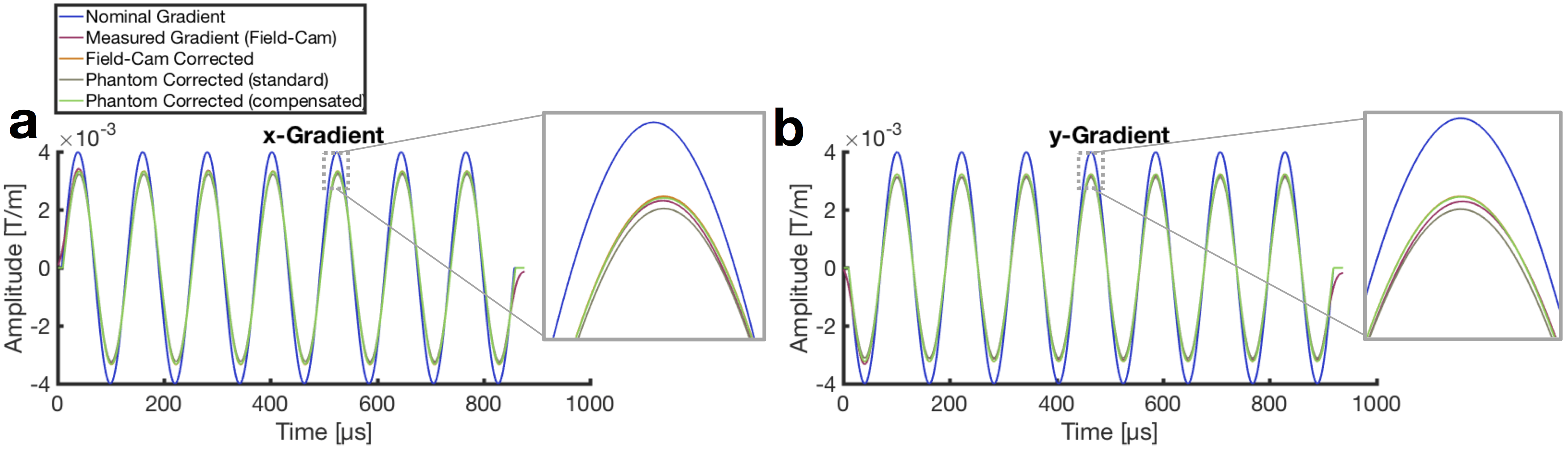
All experiments were performed on a clinical 1.5T scanner (Aera, Siemens Healthcare GmbH, Erlangen, Germany). The GSTF was determined for each gradient axis using a dynamic field camera with 16 NMR probes (Skope Medical Technologies, Zürich, Switzerland) and a standard spherical phantom. The phase responses of 12 triangular shaped input gradients (duration 100–320µs, slew rate=180T/m/s), were acquired for a prototype measurement sequence (TR=1.0s, 40 repetitions). Whereas the signal of the field camera was sampled with a fixed dwell time of $$$\tau$$$=1µs, the dwell time of the phantom measurement was varied between $$$\tau$$$=2.1-8.7µs. The acquisition duration was set to 40ms for the field camera and to 10ms for the phantom measurements. Relevant sequence parameters for the phantom-based technique were set to: slice thickness=3mm, slice positions=±16.5mm (parallel slices), flip-angle=90°. Images of a structural phantom were acquired using a 3D wave-CAIPI sequence with a 26-channel body coil. The wave-CAIPI pulse sequence featured a 3D corkscrew trajectory with a quasi-random sampling order. For the acquisition the following parameters were applied: TE=1.1ms, TR=2.5ms, flip angle=3°, slice thickness=4mm, readout=192x192x64. Sinusoidal gradient oscillations were played out on the x- and y-axes with an amplitude of 4mT/m and a frequency of ~8kHz. The GSTF-predicted gradient waveforms of both techniques were compared to the nominal gradient and measured gradient waveforms from the dynamic field camera.Results
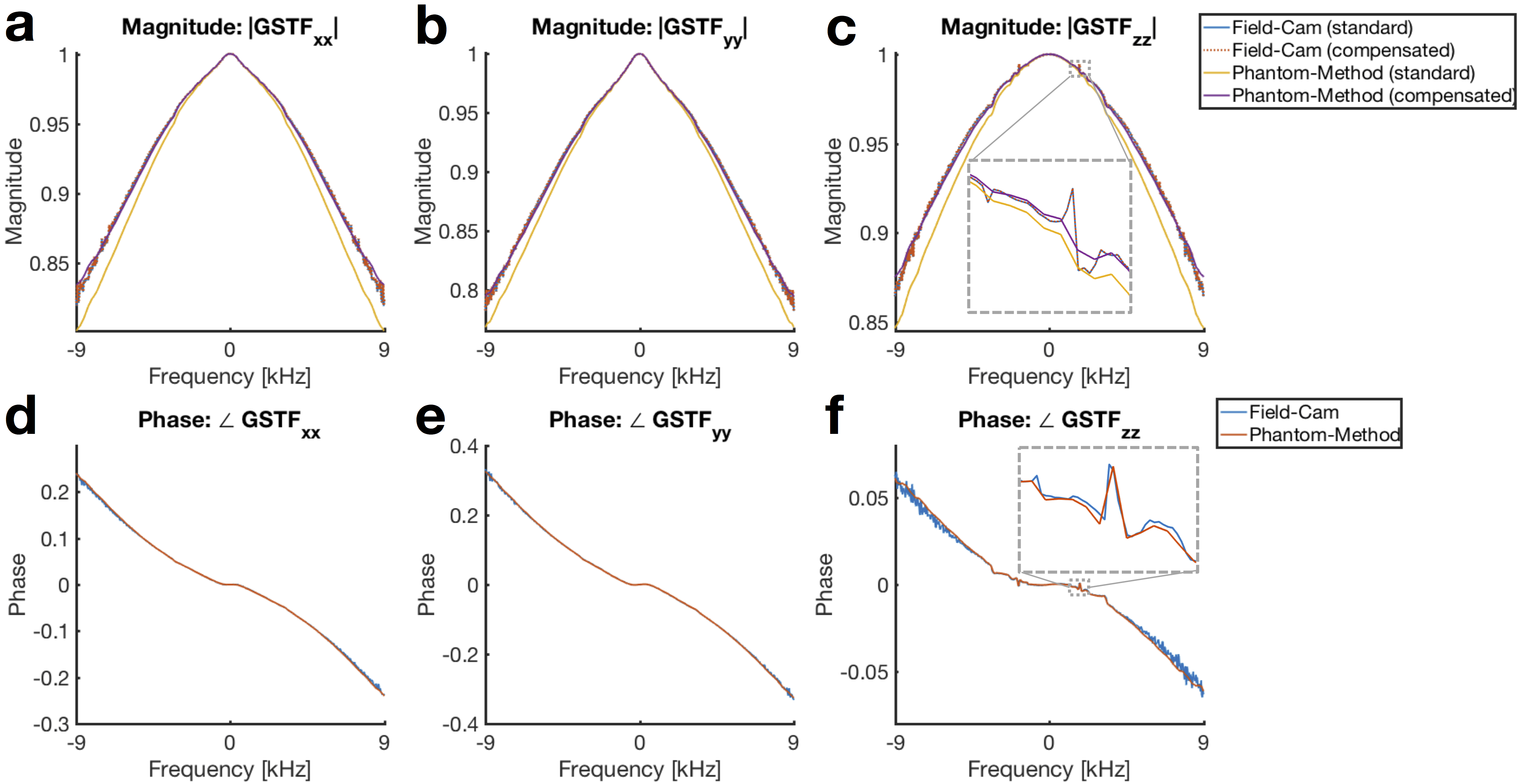
The shape of the GSTF magnitude is dependent on the scanner dwell time. Longer dwell times for the phantom measurement lead to a narrower magnitude frequency response and to a frequency transmission decline. The maximum deviation compared to the field camera GSTFs (1µs dwell time) is about 4% (at 8kHz) for a dwell time of $$$\tau$$$=8.7µs (Fig. 1a-c). When the acquisition process for a certain dwell time $$$\tau$$$ is modelled as a convolution with a box function of duration $$$\tau$$$, the influence of the dwell time can be compensated by dividing the GSTF by a sinc function, i.e. the Fourier transform of the box function. After compensating the magnitudes for the field camera and the phantom GSTFs the deviations are reduced to <0.3% (Fig. 1a-c), in contrast to the standard (uncompensated) approach. Fig. 1d-f show the phase responses for both measurement techniques with rather small deviations (<0.5%). The differences between the predicted x- and y-gradients using the phantom and field camera approach are reduced when dwell time compensation is applied (<0.5% vs ~4% deviation for the uncompensated dwell time, Fig. 2). The predicted gradient waveforms (compensated) also fit the measured gradients quite well (<1.5% deviation).
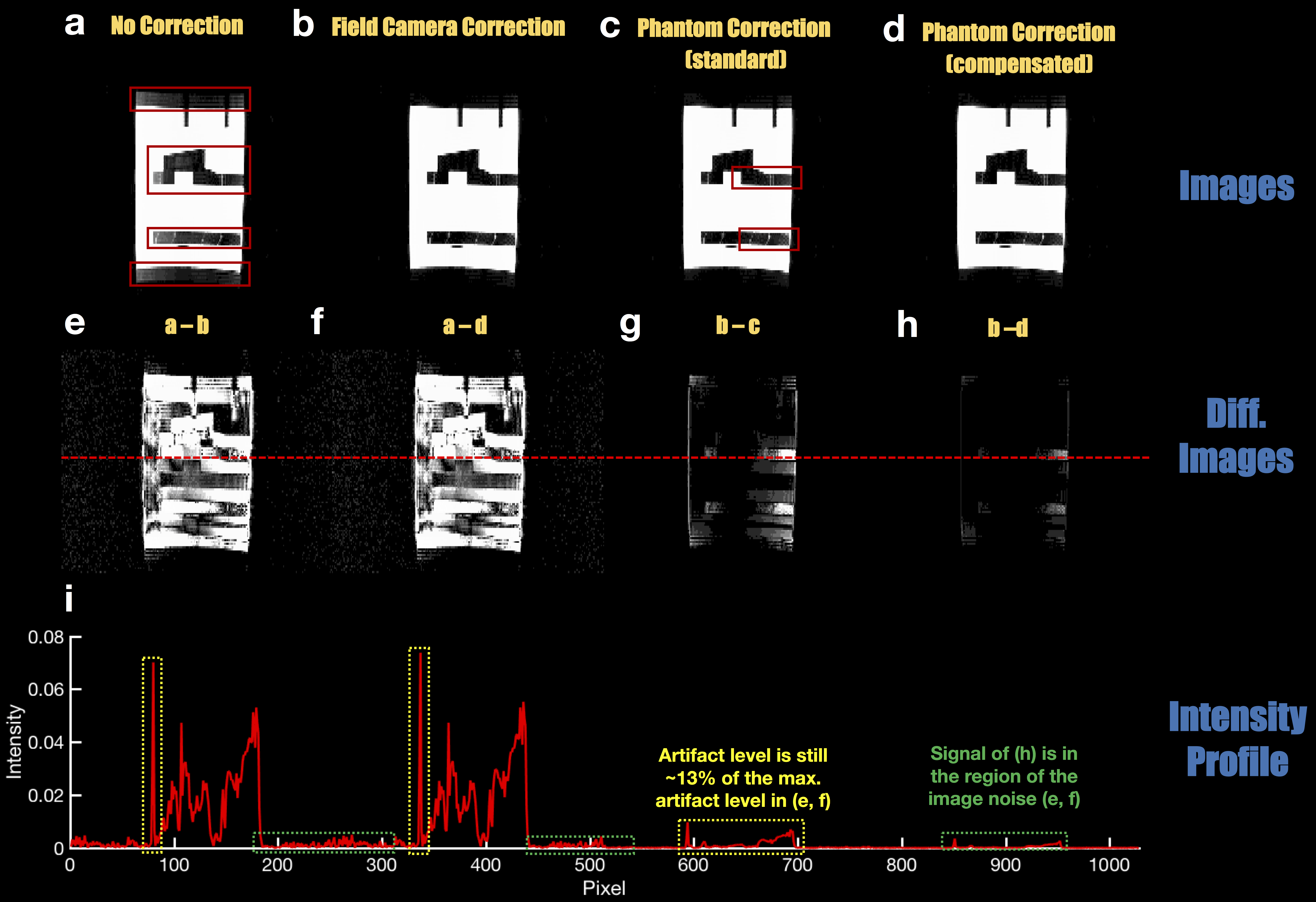
Fig. 3 shows the corresponding wave-CAIPI phantom images, reconstructed with the nominal (a), the field camera GSTF-predicted (b), the standard (c) and compensated (d) phantom GSTF-predicted trajectories. In comparison to Fig. 3a, all GSTF corrected images (Fig. 3b-d) show a well diminished artifact level. A closer look on the difference images unveils some deviations: the compensated phantom and the field camera corrected images show a better artifact suppression than the standard phantom-based correction (Fig. 3e-g,i). Fig. 3h,i visualizes, that the difference between the compensated phantom and the field camera correction is in the range of the image noise.
Discussion & Conclusion
After performing a dwell time-dependent magnitude response compensation, the GSTF magnitudes for both measurement techniques show only negligible deviations. Moreover, the phase response of the GSTFs is very similar. However, the phantom method results in a worse frequency resolution compared to the field camera. The field camera measurement was limited to 40ms acquisition to reduce noise in the GSTF. As already shown for a radial-cartesian 3D EPI sequence8, residual differences in the GSTFs are not apparent in 3D wave-CAIPI images. A dwell time-compensated phantom measurement of the GSTF is eligible to achieve the same artifact suppression as for the field camera technique. The advantage of phantom-based method is that no additional and expensive measurement hardware is needed.Acknowledgements
This work was supported by the NIH grant: Division of Intramural Research, National Heart, Lung, and Blood Institute (Z1A-HL006213, Z1A-HL006214) and the Graduate School of Life Sciences, Würzburg, Germany.
References
1. Vannesjo SJ, Haeberlin M, Kasper L, et al. Gradient system characterization by impulse response measurements with a dynamic field camera. Magn Reson Med 2013;69:583–593.
2. Duyn JH, Yang Y, Frank JA, van der Veen JW. Simple correction method for k-space trajectory deviations in MRI. J Magn Reson 1998;132:150–153.
3. Stich M, Wech T, Slawig A,et al. B0-component determination of the gradient system transfer function using standard MR scanner hardware. Joint Annual Meeting ISMRM-ESMRMB 2018. Proc. Intl. Soc. Mag. Reson. Med. 2018;26:0942.
4. Rahmer J, Marzurkewitz P, Börnert P, et al. Cross Term and Higher Order Gradient Impulse Response Function Characterization using a Phantom-based Measurement. Joint Annual Meeting ISMRM-ESMRMB 2018. Proc. Intl. Soc. Mag. Reson. Med. 2018;26:0168.
5. Campbell-Washburn AE, Xue H, Ledermann RJ, et al. Real-time distortion correction of spiral and echo planar images using the gradient system impulse response function. Magn Reson Med 2016;75:2278–2285.
6. Stich M, Wech T, Slawig A, et al. Gradient waveform pre‐emphasis based on the gradient system transfer function. Magn Reson Med 2018;80:1521–1532.
7. Bilgic B, Gagoski BA, Cauley SF, et al. Wave‐CAIPI for highly accelerated 3D imaging. Magn Reson Med 2015;73: 2152-2162.
8. Graedel NN, Hurley SA, Clare S, et al. Comparison of gradient impulse response functions measured with a dynamic field camera and a phantom-based technique. ESMRMB Congress (2017) 30 (Suppl 1): S343–S499.
Figures