0443
Temperature-dependent Gradient System Transfer Function (GSTF)1Department of Diagnostic and Interventional Radiology, University Hospital Würzburg, Würzburg, Germany, 2X-Ray & Molecular Imaging Lab, Technical University Amberg-Weiden, Weiden, Germany, 3Siemens Healthcare GmbH, Erlangen, Germany
Synopsis
The gradient system transfer function (GSTF) characterizes the frequency transfer behavior of a dynamic gradient system and can for example be used to correct non-Cartesian k-space trajectories. This work analyzes the impact of the gradient coil temperatures on the GSTF by applying gradients with high amplitudes at extensive duty cycles. The obtained results show that heating changes the transfer characteristics of the system. Based on these findings, we developed a model to predict the self- and B0-terms of the GSTF in dependency of the temperature.
Purpose
The dynamic gradient behavior of an MR scanner can be characterized by its transfer function1, which enables the correction of trajectory deviations caused by system imperfections1,2,3. However, the steady application of gradients, as it is performed for any clinical investigation, leads to heating of the system. These temperature changes affect the frequency transfer which might influence trajectory correction procedures4,5. This study investigates the temperature-dependency of the self- and B0-GSTF terms for a clinical 3T system and compares different models to calculate the temperature-dependent GSTF characteristics.Methods
Gradient heating and GSTF measurement sequence
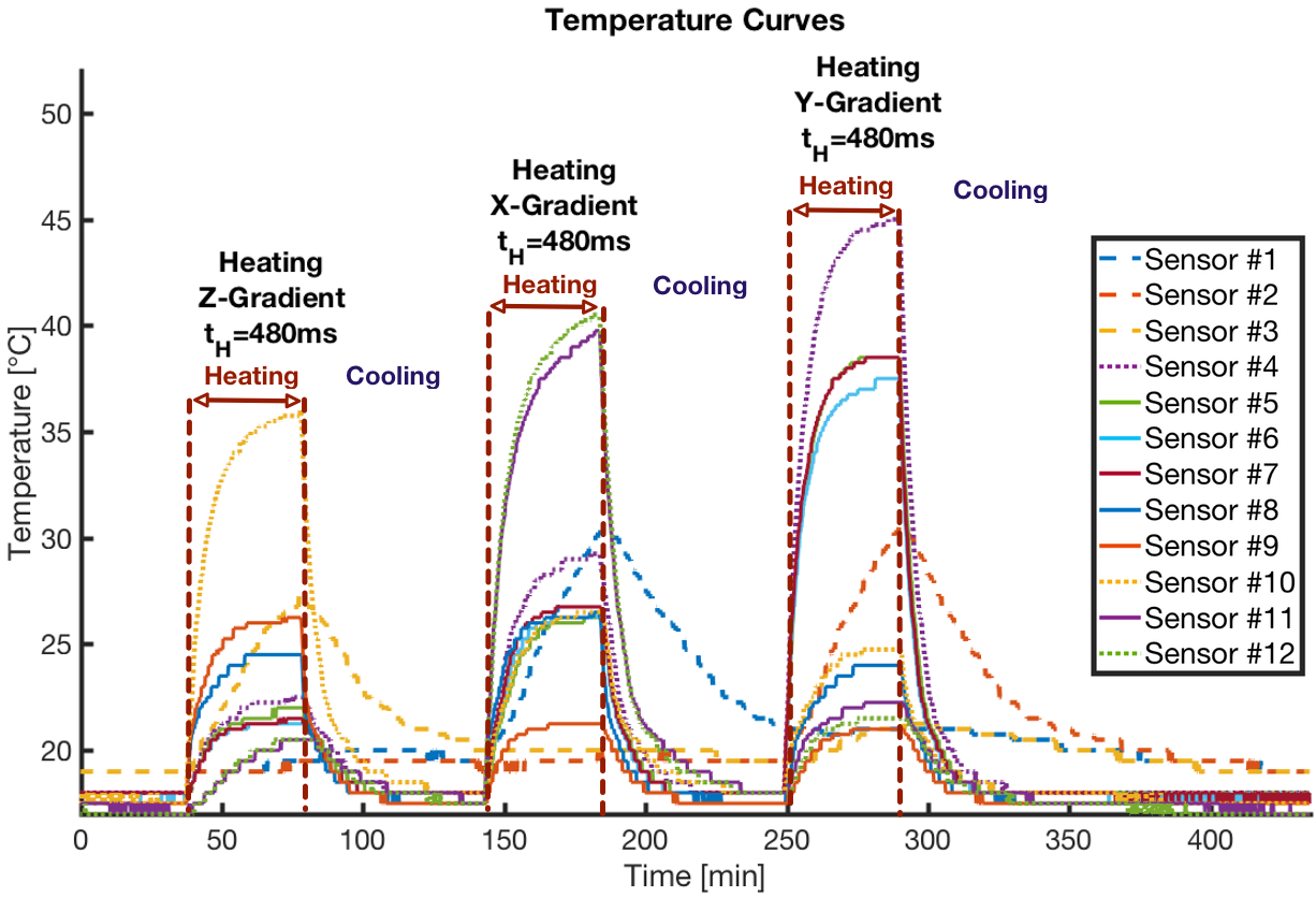
Experiments were performed using a spherical phantom placed inside a 3T MAGNETOM Skyra scanner (Siemens Healthcare, Erlangen, Germany). In a prototype sequence, 12 different triangular input gradients (duration 100–320µs, slew rate=180T/m/s) with broad spectral support were played out3,6. The responding phases were measured in two slices, vertical to the input gradient direction. Bipolar trapezoidal gradients (AH=23mT/m) were used to heat the scanner system to a steady temperature state. Other relevant measurement parameters were set to: TR=1.0s, slice thickness=3mm, slice positions=±16.5mm, flip-angle=90°, bandwidth=119kHz, 40 measurements (heating), 80 measurements (cooling). The scanner contains 12 temperature sensors, permanently integrated by the vendor at gradient connections and coils to monitor the temperature. The heating gradients were applied to different gradient axes (Fig. 1), and their duration was varied between tH=120-480ms.
Temperature-dependent GSTF models
To describe the temperature-dependent changes of the self-terms $$$\Delta{G_{self}}$$$, a linear model, with the measured input $$$I_{meas}$$$ and the model parameter $$$m$$$ was used: $$$\Delta{G_{self}}=I_{meas}\cdot{m}$$$. Two different modeling approaches were compared: A real-sensor-model (RSM), where $$$I_{meas}$$$ contains only the temperature sensor with the highest temperature contribution for the x/y/z-axis (sensor 4, 10 and 12), and in contrast to that, a virtual-sensor-model (VSM) was developed, where $$$I_{meas}$$$ consists of 1 to 12 virtual sensors resulting of a principal component analysis for all sensor combinations. Furthermore, the necessity of including the temperature derivative ($$$\dot{T}$$$) in both model approaches (RSM, VSM) was examined. For the B0-terms $$$\Delta{G_{B0}}$$$, the standard linear-model (RSM-based) was compared to a Bateman-modeling approach (RSM-based), where sensor-specific Bateman-functions ($$$b(t)=exp(-k_{1}t)-exp(-k_{2}t)$$$) were used as convolution kernels in modeling: $$$\Delta{G_{B0}}=(I_{meas}\ast{b(t)})\cdot{m}$$$. The model parameter $$$m$$$, $$$k_{1}$$$ and $$$k_{2}$$$ were fitted for all approaches using least-square minimization.
Results
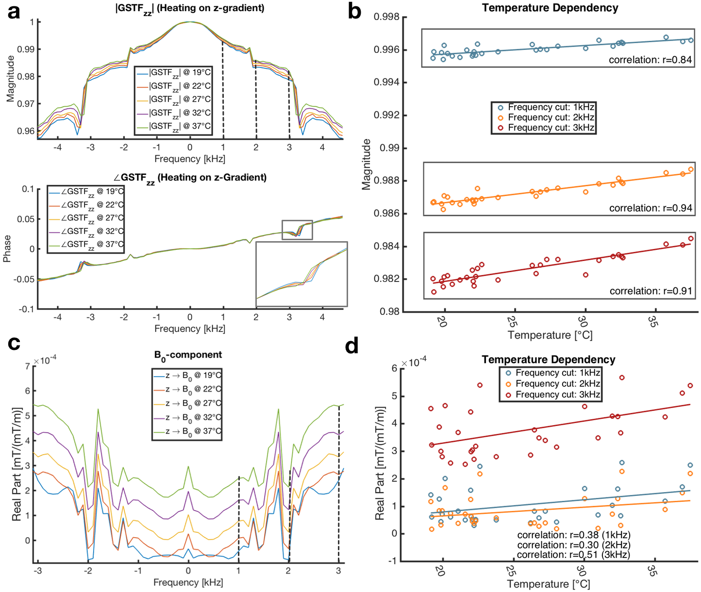
Fig. 2a shows the amplitude of GSTFzz for temperatures at the most sensitive sensor of the z-gradient coil between 19°C and 37°C. Fig. 2b displays the linear dependency of the z-self-term magnitude on the temperature. In the phase response, only mechanical resonances are slightly affected by temperature changes (Fig. 2a). For the z$$$\rightarrow$$$B0-term, the change in the magnitude is visualized in Fig. 2c. Here, magnitude and temperature do not correlate well (r<0.51, Fig. 2d).
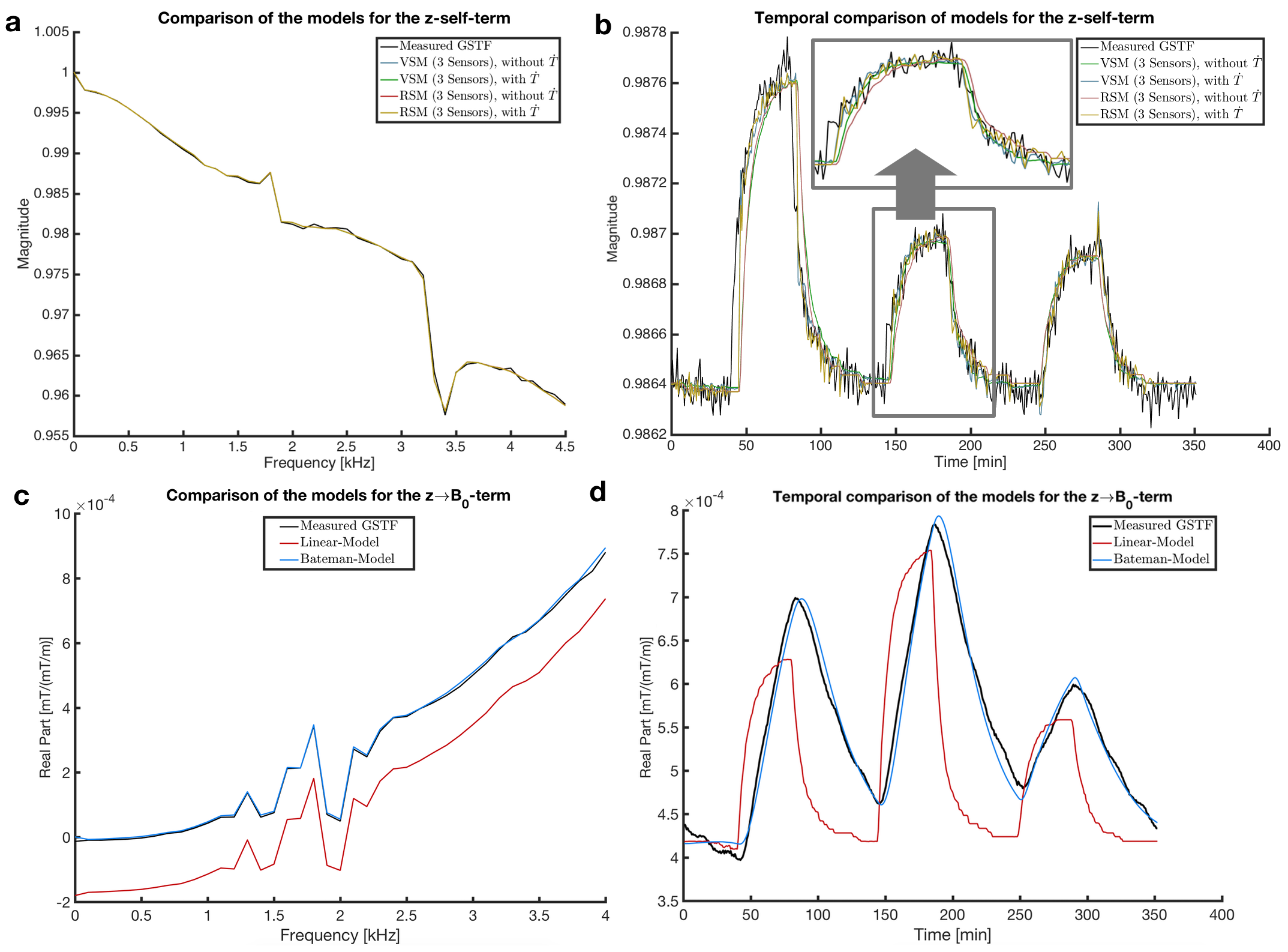
For the experiment visualized in Fig. 1 the self-term GSTF in the frequency domain (hot state, 43°C) and the temporal profile (magnitude averaged for 0-5kHz) show that the deviations between measured and modeled data are small for all approaches (Fig. 3a,b). This can also be expressed quantitatively: the goodness-of-fit $$$\chi{^2}$$$ was <0.0012 for all frequencies (sum of all temperature states). Finally, the minimum of Bayesian information criterion7 (BIC) unveils that only using three sensors with the highest temperature contribution from the x, y and z gradient coils (sensors 4, 10 and 12) is sufficient to model the GSTF ($$$\Delta$$$BIC>5). Furthermore, including the derivative of the temperature ($$$\Delta$$$BIC<1.1) is not necessary. In contrast to the self-terms, the B0-terms are not described well by a linear model (Fig. 3c,d). This is also expressed quantitively by $$$\chi{^2}$$$>2. The Bateman-modeling approach delivers good modeling results, with small values for $$$\chi{^2}$$$ (<0.0015) and $$$\Delta$$$BIC>500. The parameters $$$k_{1}$$$ and $$$k_{2}$$$ for the three Bateman-kernels are in the range of 0.05-0.29min-1 for $$$k_{1}$$$ and 0.09-0.11min-1 for $$$k_{2}$$$, respectively.
Discussion
A simple linear model using only the sensors with the highest temperature contribution from each gradient coil can be used to predict the temperature-dependency of the GSTF self-terms. In contrast to previous studies4,5, the temperature derivatives were not necessary to achieve good results which might be due to the fact that the sensors are directly integrated in the coils. For the B0-terms, heat transport has to be considered to describe the temperature response characteristics. A Bateman-model approach predicts the temperature behavior, especially at frequencies not corresponding to mechanical resonances of the system.Conclusion
This work successfully analyzes the temperature-dependency of the GSTF self- and B0-terms and develops models to predict the gradient system characteristic which fits to a current temperature state. In the future, this knowledge can be integrated in GSTF-based trajectory correction techniques1-3 to further reduce image artifacts, especially in warm temperature states.Acknowledgements
No acknowledgement found.References
1. Vannesjo SJ, Haeberlin M, Kasper L, et al. Gradient system characterization by impulse response measurements with a dynamic field camera. Magn Reson Med 2013;69:583–593.
2. Campbell-Washburn AE, Xue H, Ledermann RJ, et al. Real-time distortion correction of spiral and echo planar images using the gradient system impulse response function. Magn Reson Med 2016;75:2278–2285.
3. Stich M, Wech T, Slawig A, et al. Gradient waveform pre‐emphasis based on the gradient system transfer function. Magn Reson Med 2018;80:1521–1532.
4. Dietrich BE, Nussbaum J, Wilm BJ, Reber J and Pruessmann KP. Thermal Variation and Temperature- Based Prediction of Gradient Response. In Proc Int Soc Magn Reson Med Sci Meet Exhib, 2017, p. 0079.
5. Nussbaum J, Wilm BJ, Dietrich BE, Pruessmann KP. Improved thermal modelling and prediction of gradient response using sensor placement guided by infrared photography. In Proc Int Soc Magn Reson Med Sci Meet Exhib, 2018, p. 4210.
6. Duyn JH, Yang Y, Frank JA, van der Veen JW. Simple correction method for k-space trajectory deviations in MRI. J Magn Reson 1998;132:150–153.
7. Burnham KP, Anderson DR. Model selection and multimodal inference. A practical information-theoretic approach. New York: Springer, 2002.
Figures