0420
Biophysically motivated efficient estimation of spatially isotropic component from a single, standard gradient recalled echo measurement1Department of Systems Neuroscience, University Medical Center Hamburg-Eppendorf, Hamburg, Germany, 2Department of Neurophysics, Max Planck Institute for Human Cognitive and Brain Sciences, Leipzig, Germany, 3Department of Education and Psychology - Neurocomputation and Neuroimaging Unit, Freie Universität Berlin, Berlin, Germany, 4Paul Flechsig Institute of Brain Research, University of Leipzig, Leipzig, Germany, 5Wellcome Centre for Human Neuroimaging, UCL Institute of Neurology, London, United Kingdom
Synopsis
Gradient recalled echo-based $$$R_{2}^{*}$$$ measurements are sensitive to the degree of myelination of white matter fibres and their local orientation inside the magnetic field of the MR scanner. This orientation dependence has been observed experimentally and could be explained biophysically by anisotropic susceptibility of the myelin sheaths. In case of single, quantitative $$$R_{2}^{*}$$$ measurements the orientation dependence represents a potential confounder, since the observed $$$R_{2}^{*}$$$ would be biased by the sample’s orientation inside the scanner. Here, we propose an efficient method for separating $$$R_{2}^{*}$$$ into orientation dependent and independent components based on a biophysically motivated higher order $$$R_{2}^{*}$$$ decay model.
Introduction
$$$R_{2}^{*}$$$ measured by gradient recalled echo (GRE)
sequences is a marker depending on the myelination of fibres 1, 2,
which is also sensitive to local axonal fibre orientation $$$\theta$$$ relative
to the main magnetic field of the MR scanner 3. While this could be
used to map fibre direction using GRE measurements at multiple sample
orientations 4, 5, a single GRE measurement is biased by the
subject’s head position inside the scanner. For GRE based $$$R_{2}^{*}$$$ maps to be truly quantitative, this effect
needs to be controlled for. Here, we propose an efficient method for
decomposing $$$R_{2}^{*}$$$ into orientation independent (isotropic) and
dependent (anisotropic) components, motivated by the biophysical hollow
cylinder fibre model (HCFM), which explains orientation dependence by the
anisotropic susceptibility of myelin sheaths 5, 6. In contrast to
previous methods 4, 5, 6, 7, it requires only GRE data acquired at a
single, unknown orientation of the sample.Methods
Theory: Classically, the GRE signal is described by a mono-exponential decay, the logarithm of which may be written as a linear model
$$ ln(S(TE)) = ln(S(0)) -\beta_{1}^{(1)}TE ,\quad\quad\quad (1)$$
where $$$ln(S(0))$$$ is the signal at echo time $$$TE=0$$$ and the coefficient $$$\beta_{1}^{(1)}=R_{2}^{*}$$$ is the effective transverse relaxation time 8. Equation (1) can also be interpreted as the first order (in $$$TE$$$) approximation to a more complex signal expression as suggested in case of the HCFM 5, 6. Inspired by the second-order expansion of the predicted signal in the HCFM for TE<36 ms (at 7T) 5, we assume a quadratic signal model
$$ ln(S(TE)) = ln(S(0)) - \beta_{1}^{(2)}TE - \beta_{2}^{(2)}TE^{2} ,\quad\quad\quad (2)$$
where according to 5 $$$\beta_{1}^{(2)}$$$ is expected to be orientation independent (the isotropic component of $$$R_{2}^{*}$$$), while $$$\beta_{2}^{(2)}$$$ is expected to be orientation dependent following a $$$\sin^{4}\theta $$$-dependence (related to the anisotropic component of $$$R_{2}^{*}$$$). To validate the prediction following from the quadratic model, the orientation dependence of the components in equations (1) and (2) were investigated in an ex vivo human optic chiasm (OC), using separation of the parameters according to the well-established phenomenological model for $$$R_{2}^{*}$$$ 4, 5, 6, 7
$$\beta_{j}^{(\alpha)} = \beta_{j,iso}^{(\alpha)} + \beta_{j,aniso}^{(\alpha)}\sin^{4}\theta ,\quad\quad\quad (3)$$
with $$$\alpha =1, 2$$$ indicating model (1) or (2) and $$$j=1$$$ ($$$\alpha =1$$$) and $$$j=1, 2$$$ ($$$\alpha = 2$$$) denoting the order of the coefficient.
Sample: A human OC sample with adjoining optic nerves and tracts (OTs) was obtained at autopsy with prior informed consent (48 hrs postmortem, multiorgan failure) and approved by the responsible authorities. Following the standard Brain Bank procedures, blocks were immersion-fixed in (3% paraformaldehyde +1% glutaraldehyde) in phosphate-buffered saline.
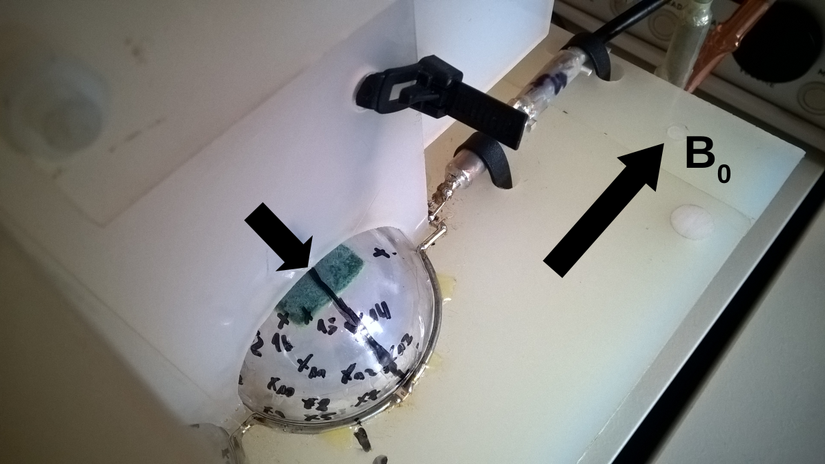
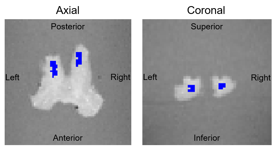
MRI: GRE measurements were performed on a 7T Siemens Magnetom MRI scanner (Siemens Healthcare, Germany) using a custom RF coil with a diameter of 60 mm and the following protocol: 16 equally spaced echoes (3.4-53.5 ms, step-size 3.34 ms), repetition time TR = 100 ms, total acquisition time: 20:59 min. The measurement was repeated 16 times, using different orientations of the sample (figure 1). The two models (1) and (2) were inverted using customized tools 9, yielding $$$\beta_{j}^{(\alpha)}$$$- maps for each angle. All parameter maps were registered to the reference. Two regions-of-interest (ROIs) in the left and right OT were manually defined (figure 2), and equation (3) was fitted to the mean signals inside the ROIs for separating $$$\beta_{j,iso}^{(\alpha)}$$$ and $$$\beta_{j,aniso}^{(\alpha)}$$$.
Results
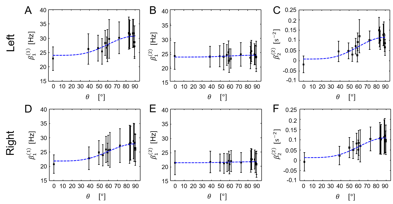
The results of the inversion according to (1) and (2) and the subsequent fits to (3) are shown in figure 3. For model (1), the well-known 4, 5, 6, 7 orientation dependence of $$$R_{2}^{*}$$$ (=$$$\beta_{1}^{(1)}$$$) was observed (figure 4). Model (2) showed orientation dependence mainly in the second-order coefficient $$$\beta_{2}^{(2)}$$$, while the first-order coefficient $$$\beta_{1}^{(2)}$$$ was orientation independent. This observation was complemented by the separation according to (3) showing that $$$\beta_{1}^{(2)}\approx\beta_{1,iso}^{(2)}$$$ and $$$\beta_{2}^{(2)}\approx\beta_{2,ansio}^{(2)}$$$ (figure 5). The anisotropic component of $$$R_{2}^{*}$$$, $$$\beta_{1,aniso}^{(1)}$$$, was in agreement with literature 4 whereas $$$\beta_{1,aniso}^{(1)}$$$ was smaller.Discussion and Conclusion
The proposed method based on inversion of (2)
allows for direct estimation of the isotropic $$$R_{2}^{*}$$$ component ($$$\beta_{1,iso}^{(1)}$$$) from
a single, standard GRE measurement in terms of $$$\beta_{1,iso}^{(2)}$$$. Moreover, the orientation dependence
of the second order in (2) suggests a direct correspondence of $$$\beta_{2}^{(2)}$$$ to
the anisotropic part of $$$R_{2}^{*}$$$. Differences in the isotropic component
of $$$R_{2}^{*}$$$ ($$$\beta_{1,iso}^{(1)}$$$ and $$$\beta_{1,iso}^{(2)}$$$) with respect to literature values 4
may be attributed to differences in the fixation protocol 10. Future
work will have to demonstrate how the proposed method translates to measurements
in vivo and at lower field strengths and validate its compatibility with
biophysical models that account for the dependence of
on
other tissue components such as iron.Acknowledgements
This work was supported by the German Research Foundation (DFG Priority Program 2041 "Computational Connectomics”, [AL 1156/2-1;GE 2967/1-1; MO 2397/5-1; MO 2249/3–1], by the Emmy Noether Stipend: MO 2397/4-1) and by the BMBF (01EW1711A and B) in the framework of ERA-NET NEURON. The research leading to these results has received funding from the European Research Council under the European Union's Seventh Framework Programme (FP7/2007-2013) / ERC grant agreement n° 616905References
- Tofts P, Quantitative MRI of the Brain: Measuring Changes Caused by Disease. John Wiley & Sons 2004
- Edwards L, Kirilina E, Mohammadi S, and Weiskopf N. Microstructural imaging of the neocortex in vivo. NeuroImage 2018; 182: 184-206
- Wiggins CJ, Gundmundsdottir V, Le Bihan D, and Chaumeil M. Orientation Dependence of White Matter $$$T_{2}^{*}$$$ Contrast at 7T: A Direct Demonstration. Proc. Intl. Soc. Mag. Reson. Med. 2008; 16: 237
- Lee J, van Gelderen P, Kuo LW, Merkle H, Silva AC, and Duyn JH. $$$T_{2}^{*}$$$–based fiber orientation mapping. NeuroImage 2011; 57: 225-234
- Wharton S, and Bowtell R. Gradient echo based fibre orientation mapping using and frequency difference measurements. NeuroImage 2013; 83: 1011-1023
- Wharton S, and Bowtell R. Fiber orientation-dependent white matter contrast in gradient echo MRI. PNAS 2012; 109(45): 18559-1856
- Gil R, Khabipova D, Zwiers M, Hilbert T, Kober T, and Marques JM. An in vivo study of the orientation-dependent and independent components of transverse relaxation rates in white matter. NMR in Biomed. 2016; 29: 1780-1790
- Bernstein M, King K, and Zhou X. Handbook of MRI Pulse Sequences. Academic Press 2007; 1st Edition
- Weiskopf N, Callaghan M, Josephs O, Antoine L, and Mohammadi S. Estimating the apparent transverse relaxation time ($$$R_{2}^{*}$$$) from images with different contrasts (ESTATICS) reduces motion artifacts. Front. Neurosc. 2014; 8: 278
- Shepherd TM, Thelwall PE, Stanisz, and Blackband SJ. Aldehyde Fixative Solutions Alter the Water Relaxation and Diffusion Properties of Nervous Tissue. MRM 2009; 62: 26 34
Figures