0342
Mapping axonal conduction velocities from in vivo MRI data1CUBRIC, Cardiff University, Cardiff, United Kingdom
Synopsis
The ability to infer axonal conduction velocities (CV) non-invasively from in vivo neuroimaging is of huge biological importance. Having previously shown that accurate CV estimates are feasible with MRI-measurable parameters, we show here the sensitivity of MRI-derived CV estimates to modelling errors and acquisition noise. We show that for the parameters typically seen in white matter axons, there is less than 5% error in CV estimates. Application to a human diffusion/relaxometry dataset generates CV estimates in corpus callosum that are close to those observed in electrophysiology literature. This illustrates further the feasibility of estimating CV from in vivo microstructural MRI.
Introduction
Being able to infer axonal conduction delays non-invasively from in vivo neuroimaging is of huge biological importance. Previously we demonstrated that a large proportion of variability of CVs can be accounted for by axon diameter and g-ratio1, for which methods for their derivation from in vivo neuroimaging already exist. However, a still unanswered question is how sensitive these measures are to modelling errors and noise. We address these issues through simulated MRI data, computing CVs from estimates of axon diameter and g-ratio and quantify the sensitivity to modelling error and MR acquisition noise. We further demonstrate the feasibility by generating a CV map of the corpus callosum from an in vivo human subject.
Method
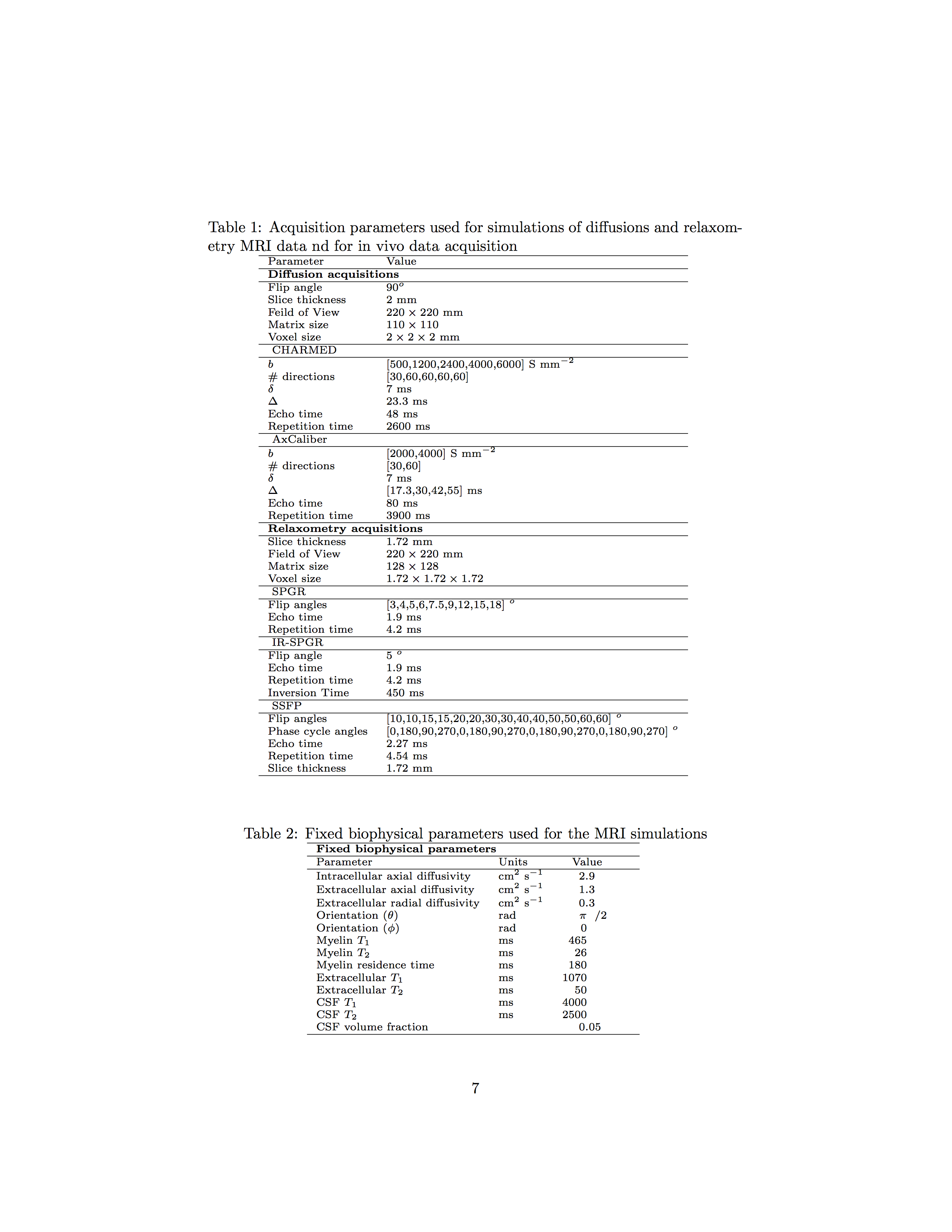
To model the effects of MR noise, MRI data was simulated using analytical expressions for three biophysical models, the CHARMED2, AxCaliber3 and mcDESPOT models4. A single population of axons with a Poisson distribution was simulated with biophysical listed in Table 2. Systems with this configuration were simulated for a range of AVFs, ADs and g-ratios. CHARMED and AxCaliber MRI data was simulated in MATLAB who parameters match a standard protocol used on a Siemens 300 mT/s Connectom system (Table 1). The simulated data was the fitted back to the CHARMED model using particle swarm global optimization5. mcDESPOT MRI data was simulated using the ’qisignal’ function in the Quantitative Imaging Toolbox (QUIT)6 and then fitted to a 3-pool model. The true MVF was estimated form the MWF using the formula:
$$\mathrm{MVF}=\frac{\mathrm{MWF}(1+\omega)}{1+\omega\mathrm{MWF}}$$
where ω=1.44 is the ratio of lipid-to-water in the myelin7. g-ratios were computed using the approach of Stikov8:
$$g=\frac{1}{\sqrt{1+\frac{\mathrm{MVF}}{\mathrm{AVF}}}}$$
CVs were estimated for each parameter combination with the Rushton model9:
$$v=pd\sqrt{-\log(g)}$$
with p=6.25 as estimated from previous simulations1. To test sensitivity
to noise, data simulations were repeated with noise s.d. at 50% and 200% of
the original noise s.d. This was done for all permutations across the 3 MRI
parameters. For all simulated acquisition and permutations of noise levels, 100
iterations were performed. This resulted in a total of 100×(1+23)×11×8=79,200 diffusion simulations and 100×(1+23)×8×12=86,400 relaxometry
simulations.
Sensitivity to bias was quantified by taking the ratio of the relative error in
CV to the relative error in the relevant imaging parameter for each model (AVF,
AD and MVF). Sensitivity to noise was estimated by taking difference in CV
estimates between the 50% and 200% noise condition and normalising to the
difference in noise s.d.
CHARMED, AxCaliber and mcDESPOT data was all acquired from a single healthy
human participant (F,28y) on a Seimens 3T 300mT/m Connectom system. The
acquisition parameters used are those used in the simulations (see Table 2). CV was calculated for the corpus callosum and bias in CV estimates were obtained by interpolating the errors from simulated model fits to appropriate points in the parameter space.
Results
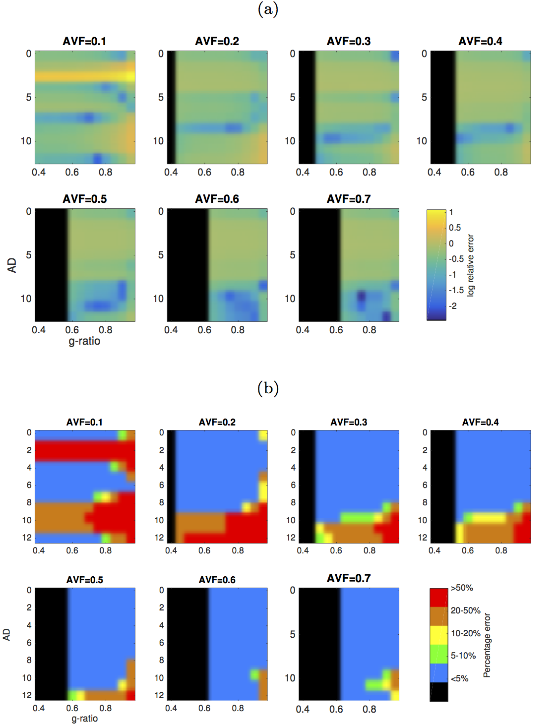
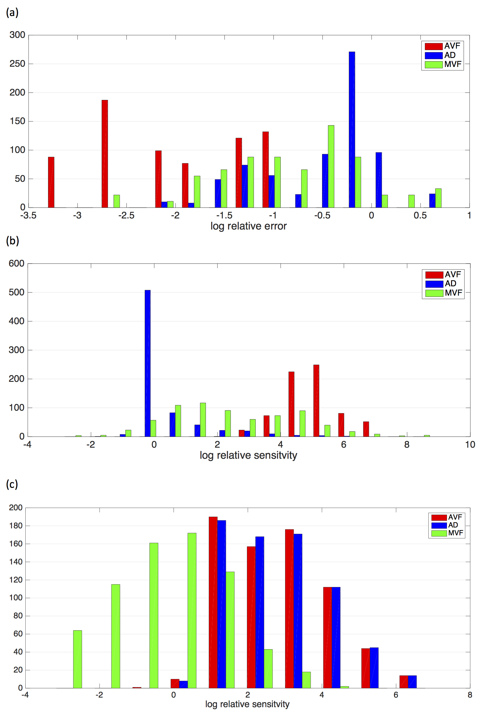
Relative errors in CV across the parameter space is shown in Figure 1. The CV estimates show a less than 5% bias across a region of parameter space where AVF is 0.25 or above, AD is below 10 μm. There is little dependency on g-ratio. Bias is worst (over 50%) in regions where AVF is low (below 0.25) and AD is low. Distributions of error of model parameters (Figure 2a) show AVF errors are overall the lowest with higher errors for MVF and AD. Relative sensitivities of model errors (Figure 2b) in AVF is much higher than for AD and MVF. Relative sensitivities to acquisition noise (Figure 2c) shows CV is less sensitive to noise in relaxometry acquisitions than for diffusion acquisitions.
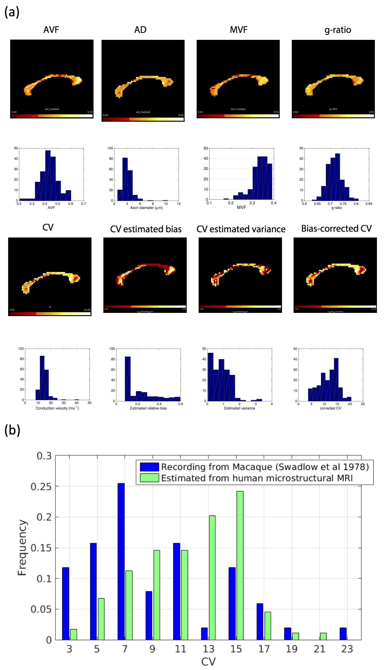
in vivo MRI data in the corpus callosum are shown in Figure 3a. CV estimates in the corpus callosum are between about 8.1-41.6 ms−1 (median:14.2 ms−1). Smaller CV estimates are seen in the genu and splenium of the corpus callosum, consistent with these regions having smaller ADs. The bias in these regions is higher than in the body of the corpus callosum. The bias-corrected CV values showed a range of 3.7-20.4 ms−1 (median: 12.2 ms−1). This is a very similar range observed from CVs estimated in Macaque corpus callosum10 (2.8-22.5 ms−1, median=7.4 ms−1, see Figure 3b).
Discussion
Overall results are that CV estimates are below 5% error over a large region of the parameter space where white-matter axons are likely to reside in. Application of the method to a in vivo dataset produced CV estimates on corpus callosum that are close to the distribution of values from direct electrophysiological measurements of CV.10 In conclusion, for g and AD values typically found in histology, this approach provides good estimate of CVs from a range of MRI approaches.Acknowledgements
This work was funded by the Wellcome Trust (grant number WT104943). We thank Tobias Wood for helpful advise on using the QUIT toolbox.References
1 M. Drakesmith and D. K. Jones, “What is the feasibility of estimating axonal conduction velocity from in vivo microstructural MRI?,” in Proceedings of the International Society for Magnetic Resonance in Medicine, (Paris, France), p. 1098, 2018.
2 Y. Assaf and P. J. Basser, “Composite hindered and restricted model of diffusion (CHARMED) MR imaging of the human brain.,” NeuroImage, vol. 27, pp. 48–58, aug 2005.
3 Y. Assaf, T. Blumenfeld-Katzir, Y. Yovel, and P. J. Basser, “AxCaliber: a method for measuring axon diameter distribution from diffusion MRI.,” Magnetic resonance in medicine, vol. 59, pp. 1347–54, jun 2008.
4 S. C. L. Deoni, B. K. Rutt, T. Arun, C. Pierpaoli, and D. K. Jones, “Gleaning multicomponent T1 and T2 information from steady-state imaging data.,” Magnetic Resonance in Medicine, vol. 60, pp. 1372–87, dec 2008.
5 J. Kennedy and R. Eberhart, “Particle swarm optimization,” Neural Networks, 1995. Proceedings., IEEE International Conference on, 1995.
6 T. C Wood, “QUIT: QUantitative Imaging Tools,” Journal of Open Source Software, vol. 3, p. 656, jun 2018.
7 D. Agrawal, R. Hawk, R. L. Avila, H. Inouye, and D. A. Kirschner, “Internodal myelination during development quantitated using X-ray diffraction,” Journal of Structural Biology, vol. 168, no. 3, pp. 521–526, 2009.
8 N. Stikov, J. S. Campbell, T. Stroh, M. Lavelée, S. Frey, J. Novek, S. Nuara, M.-K. K. Ho, B. J. Bedell, R. F. Dougherty, I. R. Leppert, M. Boudreau, S. Narayanan, T. Duval, J. Cohen-Adad, P.-A. A. Picard, A. Gasecka, D. Côté, and G. B. Pike, “In vivo histology of the myelin g-ratio with magnetic resonance imaging,” NeuroImage, vol. 118, pp. 397–405, sep 2015.
9 W. A. H. Rushton, “A theory of the effects of fibre size in medullated nerve,” The Journal of Physiology, vol. 115, pp. 101–122, sep 1951.
10 H. Swadlow, D. Rosene, and S. Waxman, “Characteristics of interhemispheric impulse conduction between prelunate gyri of the rhesus monkey,” Experimental Brain Research, vol. 33, no. 3-4, 1978.
Figures