0324
Artifact free direct conductivity reconstruction method using the Dual Loop and artificial neural network with one current injection in MREIT.1School of Biological and Health Systems Engineering, Arizona State University, Tempe, AZ, United States
Synopsis
Most the image reconstruction algorithms in magnetic resonance electrical impedance tomography (MREIT) and diffusion tensor magnetic resonance electrical impedance tomography (DT-MREIT) require at least two independent current patterns to uniquely reconstruct conductivity distributions. However, in transcranial electrical current stimulation (tES) or deep brain stimulation (DBS) only one current injection data is available. We applied Kirchhoff’s voltage law (KVL) in a mimetic discretized network, additional current data obtained from a computational model, and a radial basis function artificial neural network (RBF-ANN) approach, to demonstrate that it is possible to reconstruct the conductivity images using a single experimental current administration.
INTRODUCTION
To probe tissue electrical properties using MREIT or DT-MREIT technique, a low intensity current is applied using a pair of electrodes and one component of the magnetic flux density data ($$$B_z$$$) is collected using a MRI scanner1-2. While current density can be estimated from one set of $$$B_z$$$ data, stable conductivity reconstruction requires two independent current administrations1-2. Lee et al.3 used one current profile data to reconstruct conductivity image from known conductivity values at the boundary using the KVL in a mimetic discretized network. However, the performance of the reconstructed images was limited due to streaking artifact caused by the noise propagation along equipotential lines3. Therefore, until now MREIT/DT-MREIT technique could not be used to reconstruct ‘apparent’ tissue conductivities during tES/DBS studies. We used additional $$$B_z$$$ data obtained from a computational model and RBF-ANN correction in this work to demonstrate the feasibility of conductivity reconstruction using one experimental current injection.METHODS
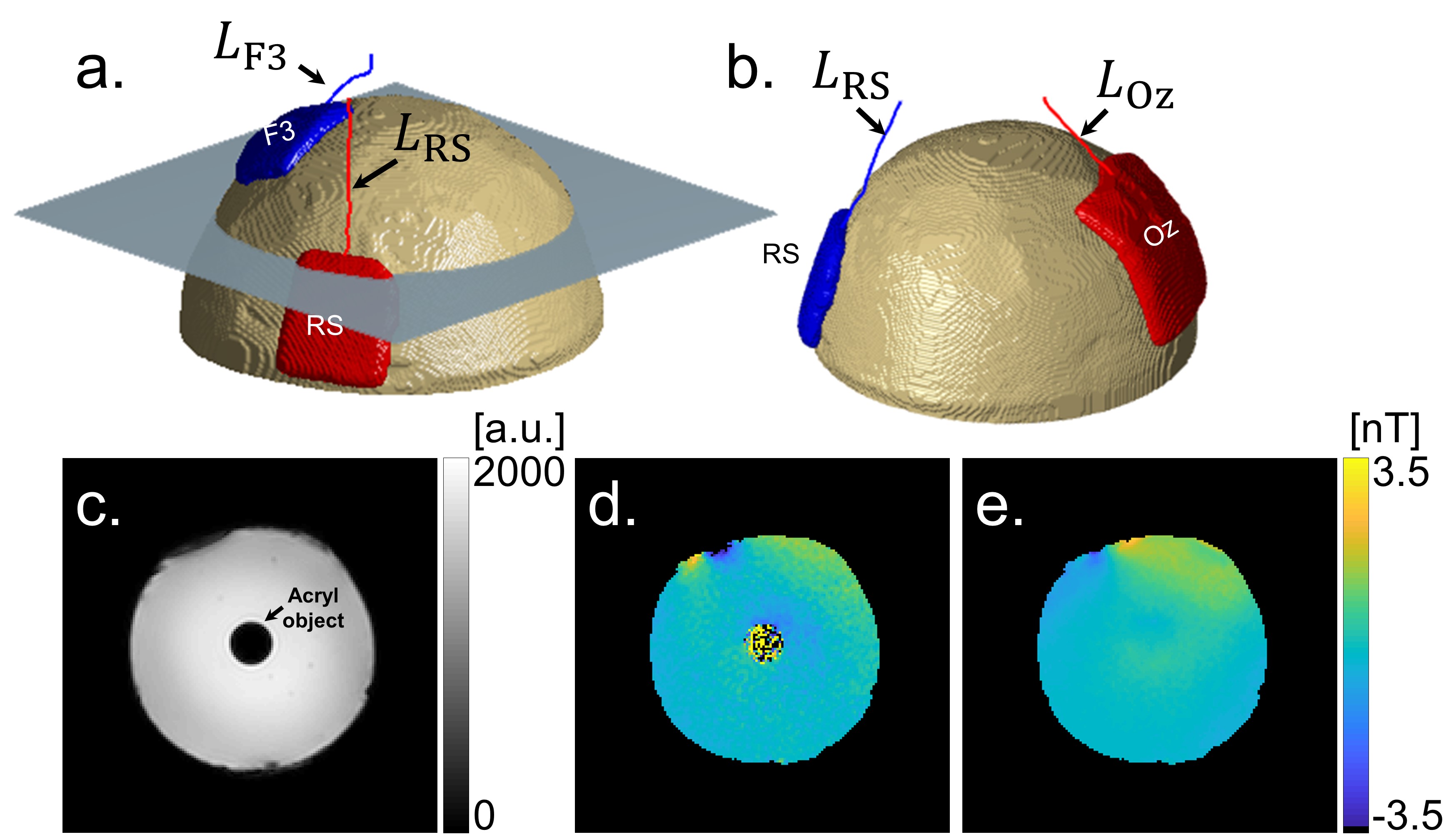
Experiment: A hemispheric phantom composed with agar-gel (1 S/m) was used in this study (Fig. 1a). A cylindrical shaped acrylic object was placed inside the phantom to provide contrast (Fig-1c). A pair of carbon electrodes were attached on the surface of the phantom at F3 and RS locations (Fig. 1a). All data were measured using a 32-channel head coil and the 3.0T Ingenia Philips MRI scanner located at the Barrow Neurological Institute, Phoenix, Arizona, USA. Using the protocol for human tES study2 we performed the MREIT experiment with 1.5 mA current injection. Three slices of data were collected at voxel size 1.5x1.5x5 mm3 using 160 phase encoding steps. The other parameters were, TR/TE = 50/7ms, NE = 10, ES = 3ms NEX = 24. High resolution T1-weighted images were also collected to construct a computational model of the phantom and lead wires (Fig. 1a). The imaging domain contained a signal void region from the acrylic object (Fig. 1c). Inclusion of this ROI during parameter reconstruction deteriorates quality of the reconstructed image4. Therefore, we inpainted1 the $$$B_z$$$ signal within this anomaly in each echo after stray field correction. Echo images were then combined using the method proposed by Kim et al.5 (Fig. 1e).
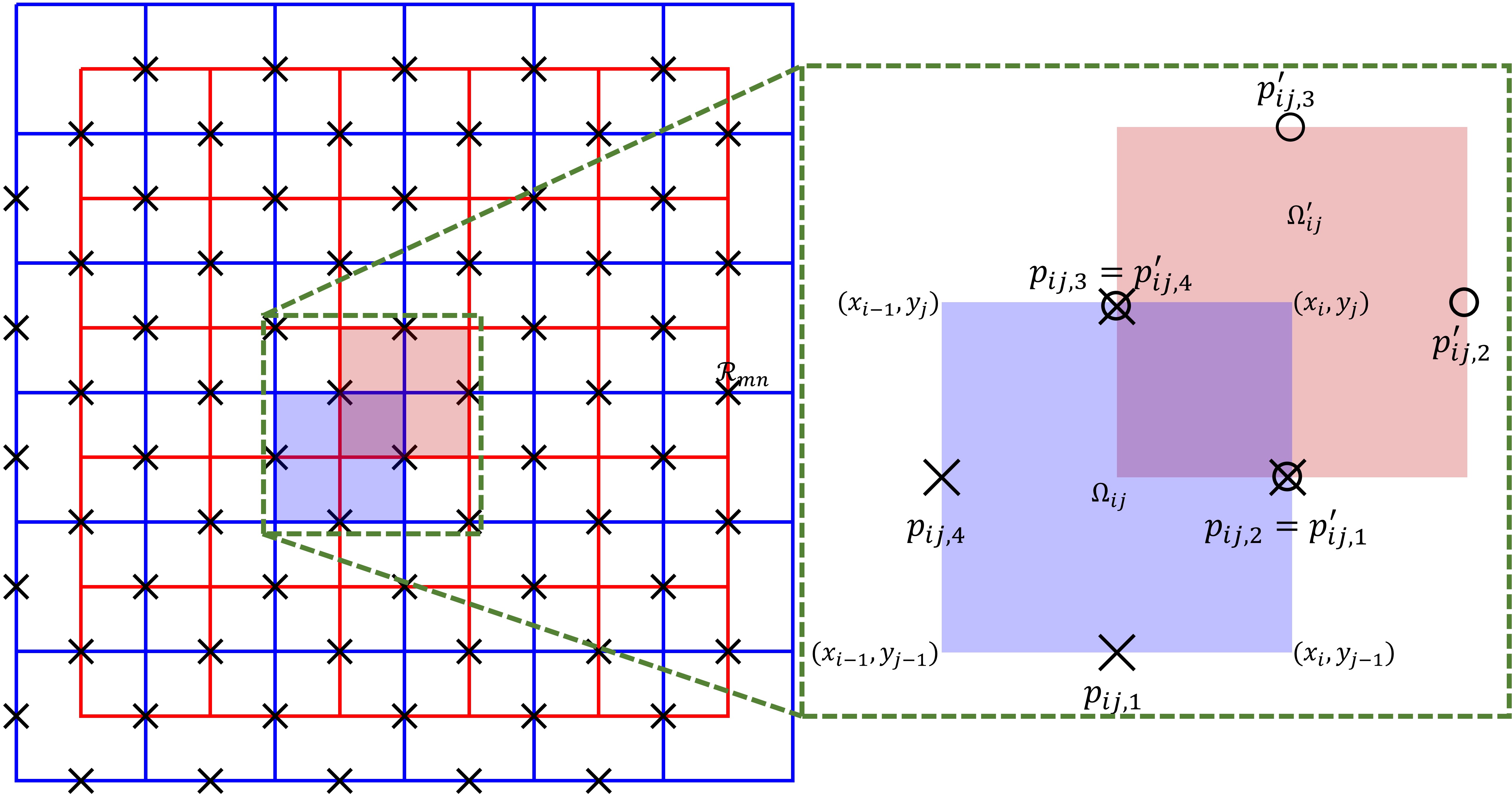
Image reconstruction: Applying KVL in an arbitrary rectangular region $$$\Omega_{i,j},\Omega^{'}_{i,j} \in \Omega_{t} $$$ where, $$$\Omega_t$$$ is the collected MREIT slices at plane Lee et al.3 (Fig. 2) formulate,
$$\begin{cases}\frac{J^p_x(p_{ij,1})}{\sigma(x_i,y_{j-1})}+\frac{J^p_y(p_{ij,2})}{\sigma(x_i,y_j)}-\frac{J^p_x(p_{ij,3})}{\sigma(x_i,y_j)}-\frac{J^p_y(p_{ij,4})}{\sigma(x_{i-1},y_j)} = 0 ~~~in~\Omega_{ij} \\\frac{J^p_x(p^{'}_{ij,1})}{\sigma(x_i,y_j)}+\frac{J^p_y(p^{'}_{ij,2})}{\sigma(x_{i+1},y_j)}-\frac{J^p_x(p^{'}_{ij,3})}{\sigma(x_i,y_{j+1})}-\frac{J^p_x(p^{'}_{ij,4})}{\sigma(x_i,y_j)}= 0 ~~~in~\Omega^{'}_{ij}\end{cases}~~~~ (1)$$
where, $$$\mathbf{J}^p$$$ is estimated projected current density4. With known boundary conductivity values, an overdetermined system was built comprising $$$2(N-2)^2$$$ equations, which was then solved for $$$(N-2)^2$$$ internal nodes. Since the reliability of the reconstructed image was limited due to streaking artifacts3, a RBF-ANN was trained using 100 numerical models (agar: 0.7-1.4, anomaly: 0.5-1.0 S/m with 0.1 S/m linear step) using the RS-F3 electrode montage, with the assumption that conductivity was piece-wise constant in each ROI. Prior to calculating datasets from equation (1), estimated noise6 (0.18 nT for RS-F3) was added to each simulated $$$B_z^{*}$$$ image. Data from a complementary electrode montage (Oz-Rs) was simulated (Fig. 1b). We obtained the output datasets from this second set of data $$$\tilde{B}_z^*$$$ as4,
$$\begin{array}{llll}\begin{bmatrix}J^{p*}_y & -J^{p*}_x \\\tilde{J}^{p*}_y & -\tilde{J}^{p*}_x \end{bmatrix}\end{array}\begin{array}{llll}\begin{bmatrix}\frac{\partial\sigma}{\partial x} \\\frac{\partial\sigma}{\partial y} \end{bmatrix}\end{array}=\begin{array}{llll}\begin{bmatrix}\frac{\partial J^{p,*}_x}{\partial y}-\frac{\partial J^{p,*}_y}{\partial x} \\\frac{\partial \tilde{J}^{p,*}_x}{\partial y}-\frac{\partial \tilde{J}^{p,*}_y}{\partial x} \end{bmatrix}\end{array} ~~~~~(2)$$
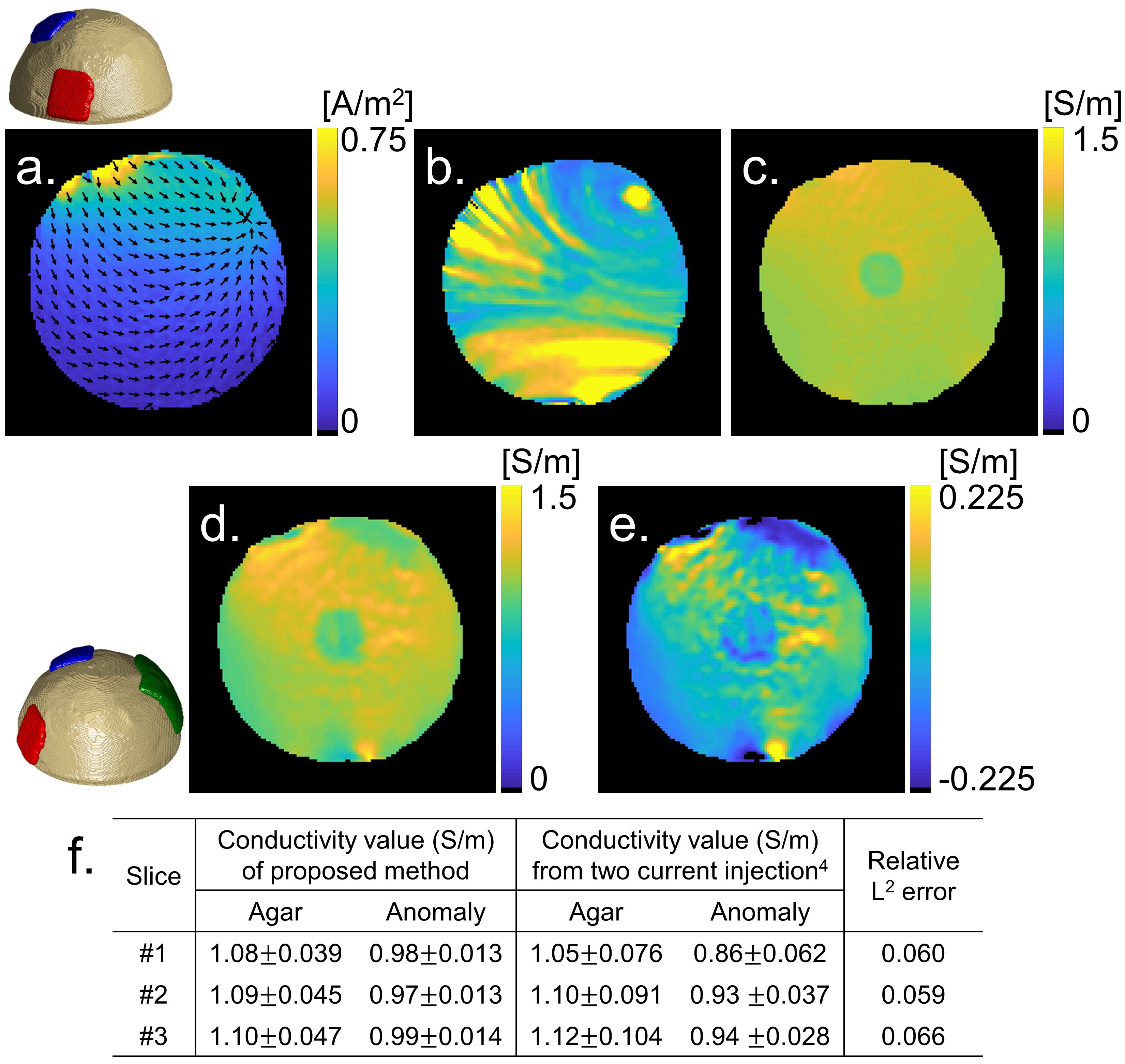
Verification: We also measured another set of $$$\tilde{B}_z$$$ data caused due to the 1.5 mA current flowing through the Oz-RS electrode pair as shown in figure 1(b). To verify reconstruction performance, we solved the matrix system in (2) using the $$$B_z,~\tilde{B}_z$$$ datasets and relative L2 errors were measured between the proposed and standard two current injection method4.
RESULTS
Figure 1(a) shows the estimated projected current density caused by current flow through the RS-F3 electrode pair. We reconstructed the conductivity using equation (1) with known boundary conductivity value (1 S/m) (Fig. 1b). As expected, reconstructed conductivity image from one current injection was corrupted by streaking artifacts. Results obtained after correction using the ANN trained with 30 hidden-layers is displayed in figure 3(c) and compared with those from the two current administration method4 (Fig. 3d-f).DISCUSSION
We present an image artifact correction method for dual-loop algorithm3 using RBF-ANN. The present method can easily be extended to obtain scale factor reconstructions to solve full conductivity tensors using DT-MREIT2. One of the drawbacks of RBF-ANN is that it only works with model specific training datasets. To avoid this shortcoming, we plan to extend this approach using deep learning methods.CONCLUSIONS
Result from the simple hemispheric phantom presented in this work demonstrate that it is possible to reconstruct stable current density and conductivity tensor data from one current injection.Acknowledgements
This work was supported by award RF1MH114290 to RJS.References
1. Woo E J and Seo J K. Magnetic resonance electrical impedance tomography (MREIT) for high-resolution conductivity imaging. Physiol Meas., 2008; 29(10): R1-26.
2. Chauhan M, Indahlastari A, Kasinadhuni A, et al. Low-frequency conductivity tensor imaging of the human head in-vivo using DT-MEIT: first study. IEEE Trans. Med. Imaging 2018; 37 (4): 966-76.
3. Lee T H, Nam H S, Lee M G et al. Reconstruction of conductivity using dual-loop method with one injection current in MREIT. Phys. Med. Biol. 2010; 55 (24): 7523-39 (2010).
4. Sajib S Z K, Kim H J, Kwon O I et al. Regional absolute conductivity reconstruction using projected current density in MREIT. Phys. Med. Biol. 2012; 57 (18):5841-59.
5. Kim M N, Ha T Y, Woo E J et al. Improved conductivity reconstruction from muti-echo MREIT utilizing weighted voxel-specific signal-to-noise ratios. Phys. Med. Biol. 2012; 57 (11):3643-59.
6. Sadleir R J, Grant S, Zhang S U et al. Noise analysis in MREIT at 3 and 11 Tesla field strength. Physiol. Meas. 2005; 27(5):875-84.
Figures