0322
One-Dimensional k-Space Metrics on Cone Surfaces for Quantitative Susceptibility Mapping1Department of Diagnostic and Interventional Radiology, Technical University of Munich, Munich, Germany, 2Philips Research, Hamburg, Germany, 3Department of Electrical Engineering and Computer Sciences, & Helen Wills Neuroscience Institute, University of California, Berkeley, Berkeley, CA, United States
Synopsis
An important question in QSM is how to compare different QSM reconstructions. We propose new metrics to compare susceptibility maps on cone surfaces in the Fourier domain following the intrinsic geometry of the dipole kernel. This physically motivated approach augments the idea of previously proposed error spectrum plots in MRI image reconstruction to specifically suit the QSM dipole inversion. The novel metrics complement previous metrics used in the 2016 QSM reconstruction challenge.
Introduction
Dipole inversion is the last algorithmic step in QSM1. The forward model to this inverse field-to-susceptibility problem is described by a convolution of the susceptibility distribution with a dipole kernel. To efficiently solve the inverse de-convolution, the problem is mapped to k-space2. The dipole-kernel in k-space is zero on the cone surface—further referred to as Zero Cone Surface (ZCS)—at the azimuthal (magic) angle of $$$~54.7^\circ$$$. Therefore, dipole inversion is an ill-posed problem and requires regularization.
In the past many QSM regularization techniques have been developed. In 2016 a QSM reconstruction challenge was initiated to investigate the performance of the plethora of methods3. By using results of multi-orientation QSM as the reference, a major challenge was to find quantitative metrics to compare different QSM methods.
The employed metrics promoted susceptibility maps that showed significant discrepancy to what a visual human comparison would favor. Generally, these metrics are scalar quantities not specific to QSM and difficult to develop an intuitive understanding from them.
In the field of MRI image reconstruction, a method called the Error Spectrum Plot (ESP) was previously proposed to compare and ultimately combine different reconstruction results4,5. ESP compares the Fourier transform of images on spherical surfaces at different radii and therefore gains information about where in the k-space two reconstructions differ the most.
We adopt the ESP concept and translate it to the intrinsic cone geometry of the dipole inversion problem in QSM. The resulting novel one-dimensional metrics are used to compare dipole inversion techniques, to intuitively understand the effect of morphological priors in the regularization and to guide selection of hyper parameters.
Methods
Assuming the dipole inversion as the optimization problem
$$\text{min}_X||\Psi-DX||_2+\lambda R(X),\quad(1)$$
with magnetic field $$$\Psi$$$, dipole kernel $$$D=1/3-k^2_z/|\vec{k}|^2$$$, and susceptibility $$$X$$$, all in k-space where the main magnetic field points along the \(\hat{z}\)-axis. $$$R(X)$$$ is the regularization term. The resulting susceptibility map is given by the inverse Fourier transform $$$\chi=\text{FT}^{-1}(\text{reshape}(X))$$$.
Theory
Given two dipole inversion results $$$\chi_1$$$ and $$$\chi_2$$$, the original ESP relates values on spherical surfaces of different radii in k-space by computing the "error spectrum" see Equation $$$(2)$$$ in Figure 1, where the spherical surface is parameterized by $$\omega_r\in\Omega_r=\left\{\omega\Big|\omega(\vec{k})=|\vec{k}|\right\}.\quad(3)$$
Following the same concept, we compute normalized errors on two additional surface parameterizations in k-space:
- cone surfaces of different azimuthal angle $$$\theta$$$: $$\Omega_\theta=\left\{\omega\Big|\omega(\vec{k})=\theta=\arccos\left(k_z/|\vec{k}|\right)\right\},\quad(4)$$
- and k-space regions of different Euclidean distance to the ZCS with $$$\theta_{\dagger}=\pi/2-\arccos\left(1/\sqrt{3}\right)\approx 54.7^{\circ}$$$, $$\Omega_d=\left\{\omega\Big|\omega(\vec{k})=d=|\vec{k}|\sin\left(\theta_{\dagger}\pm\theta\right)\right\}.\quad(5)$$
These surfaces, depicted in Figure 1, follow the geometry dictated by the dipole-kernel in Equation (1). Figure 2 shows how susceptibility comparison on these k-space surfaces is implemented.
QSM reconstruction challenge
The three different one-dimensional metrics above were computed for the publicly available data from the 2016 QSM reconstruction challenge3. The baseline QSM reconstructions of TKD6, L2-regularized closed form solution7, and COSMOS8 were compared to the STI result ($$$\chi_{33}$$$)9,10.
Numerical phantom study
Using the metrics on a numerical brain phantom, the introduction of morphological edge weights $$$M$$$ in the regularizer $$$R=||M\nabla\chi||_2$$$ of Eq. (1) —as done in the state-of-the-art Morphology-Enabled Dipole Inversion (MEDI) technique11— was studied.
Furthermore, we employed the one-dimensional metrics for the selection of the regularization parameter $$$\lambda$$$ in the same MEDI technique.
Results
Figure 3 compares the TKD6, L27, and COSMOS8 to $$$\chi_{33}$$$9 using the proposed metrics. Arrows indicate the metrics' potential to visualize fundamental difference in the dipole inversion methods: In TKD, dipole kernel values at azimuthal angles close to the magic angle are altered which results in lower errors on cone surfaces around $$$\theta=\theta_{\dagger}$$$ (blue profile, bottom row, middle).
Figure 4 shows QSM results for a numerical brain phantom with and without a morphological edge weighting in the gradient-based MEDI regularization term. The 1D metrics reveal how the edge weighting reduces the error in k-space regions far from the zero cone surface at the cost of an increased bias in susceptibility contrast as can be seen by the larger errors close to the ZCS.
Figure 5 demonstrates how the 1D metrics can be useful for hyper parameter tuning. Stronger regularization reduces errors close to the ZCS. Errors in the k-space periphery can identify unfeasible parameters.
Discussion/Conclusion
1D metrics on parameterized cone surfaces result in interpretable comparisons between different dipole inversion techniques based on the physics of the inverse problem and the well-established concept of k-space.
In the original ESP method the parameterized spherical surfaces allow for an intuitive method to fuse different reconstructions and their combine advantages. Potential limitation of this approach in QSM due to absent DC reference needs to be further assessed.
Results from the application of the proposed metrics can also help in the design of novel noise damping filters in k-space based on the same concept of distance to the ZCS.
Acknowledgements
The present work was supported by the European Research Council (grant agreement No 677661 – ProFatMRI) and Philips Healthcare.
This work reflects only the authors view and the EU is not responsible for any use that may be made of the information it contains.
The software used for this work will be freely available at http://bmrrgroup.de/software/.
References
[1] Wang, Y., & Liu, T., Quantitative susceptibility mapping (qsm): decoding mri data for a tissue magnetic biomarker, Magnetic Resonance in Medicine, 73(1), 82–101 (2014). http://dx.doi.org/10.1002/mrm.25358
[2] Marques, J., & Bowtell, R., Application of a fourier-based method for rapid calculation of field inhomogeneity due to spatial variation of magnetic susceptibility, Concepts in Magnetic Resonance Part B: Magnetic Resonance Engineering, 25B(1), 65–78 (2005). http://dx.doi.org/10.1002/cmr.b.20034
[3] Langkammer, C., Schweser, F., Shmueli, K., Kames, C., Li, X., Guo, L., Milovic, C., …, Quantitative susceptibility mapping: report from the 2016 reconstruction challenge, Magnetic Resonance in Medicine, 79(3), 1661–1673 (2017). http://dx.doi.org/10.1002/mrm.26830
[4] Kim, T. H., & Haldar, J. P., The fourier radial error spectrum plot: a more nuanced quantitative evaluation of image reconstruction quality, In , 2018 IEEE 15th International Symposium on Biomedical Imaging (ISBI 2018)
[5] Kim, T. H., & Haldar, J. P., Assessing mr image reconstruction quality using the fourier radial error spectrum plot, In , Proceedings 26. Annual Meeting International Society for Magnetic Resonance in Medicine (pp. 0249) (2018). Paris, France: http://archive.ismrm.org/2018/0249.html
[6] Shmueli, K., Zwart, J. A. d., Gelderen, P. v., Li, T., Dodd, S. J., & Duyn, J. H., Magnetic susceptibility mapping of brain tissue in vivo using mri phase data, Magnetic Resonance in Medicine, 62(6), 1510–1522 (2009). http://dx.doi.org/10.1002/mrm.22135
[7] Bilgic, B., Chatnuntawech, I., Fan, A. P., Setsompop, K., Cauley, S. F., Wald, L. L., & Adalsteinsson, E., Fast image reconstruction with l2-regularization, Journal of Magnetic Resonance Imaging, 40(1), 181–191 (2013). http://dx.doi.org/10.1002/jmri.24365
[8] Liu, T., Spincemaille, P., Rochefort, L. d., Kressler, B., & Wang, Y., Calculation of susceptibility through multiple orientation sampling (cosmos): a method for conditioning the inverse problem from measured magnetic field map to susceptibility source image in mri, Magnetic Resonance in Medicine, 61(1), 196–204 (2009). http://dx.doi.org/10.1002/mrm.21828
[9] Liu, C., Susceptibility Tensor Imaging, Magnetic Resonance in Medicine, 63(6), 1471–1477 (2010). http://dx.doi.org/10.1002/mrm.22482
[10] Li, W., Wu, B., & Liu, C., STI suite: a software package for quantitative susceptibility imaging, In , Proceedings 22. Annual Meeting International Society for Magnetic Resonance in Medicine (pp. 3265) (2014). Milan, Italy: http://archive.ismrm.org/2014/3265.html.
[11] Liu, T., Xu, W., Spincemaille, P., Avestimehr, A. S., & Wang, Y., Accuracy of the morphology enabled dipole inversion (medi) algorithm for quantitative susceptibility mapping in mri, IEEE Transactions on Medical Imaging, 31(3), 816–824 (2012). http://dx.doi.org/10.1109/tmi.2011.2182523
Figures
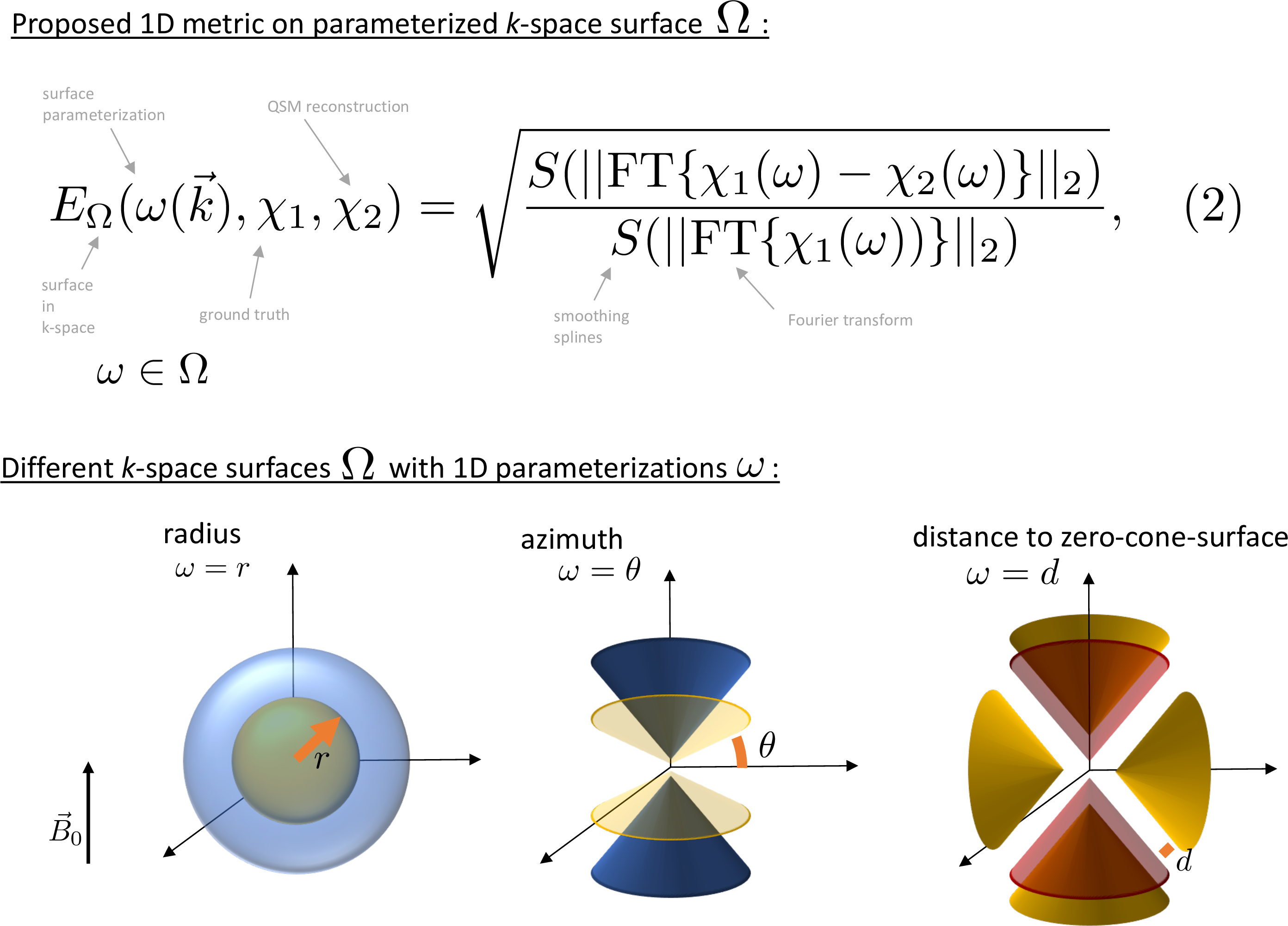
Figure 1: Top: Main Equation (2) to compute one-dimensional error metrics on parameterized surfaces in k-space. Bottom: Different regions of the Fourier domain and their one-dimensional parameterizations (Equations $$$(3)$$$–$$$(5)$$$) on which susceptibility maps are compared.
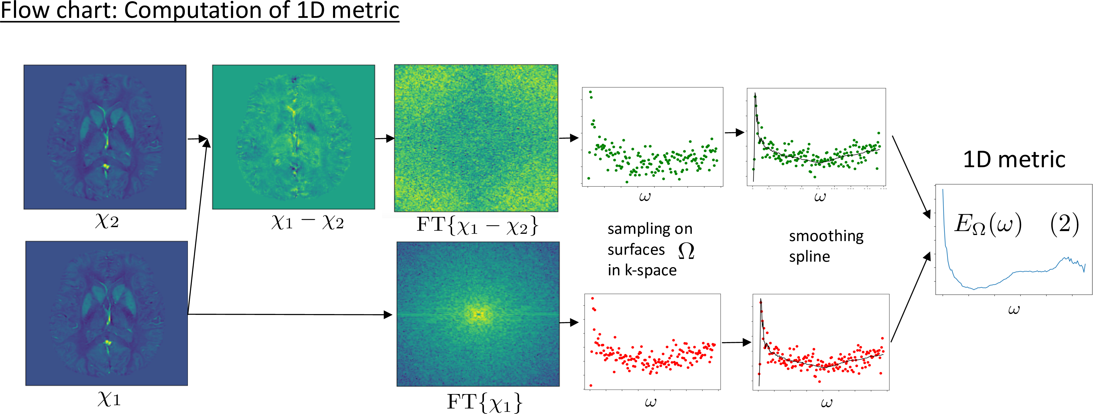
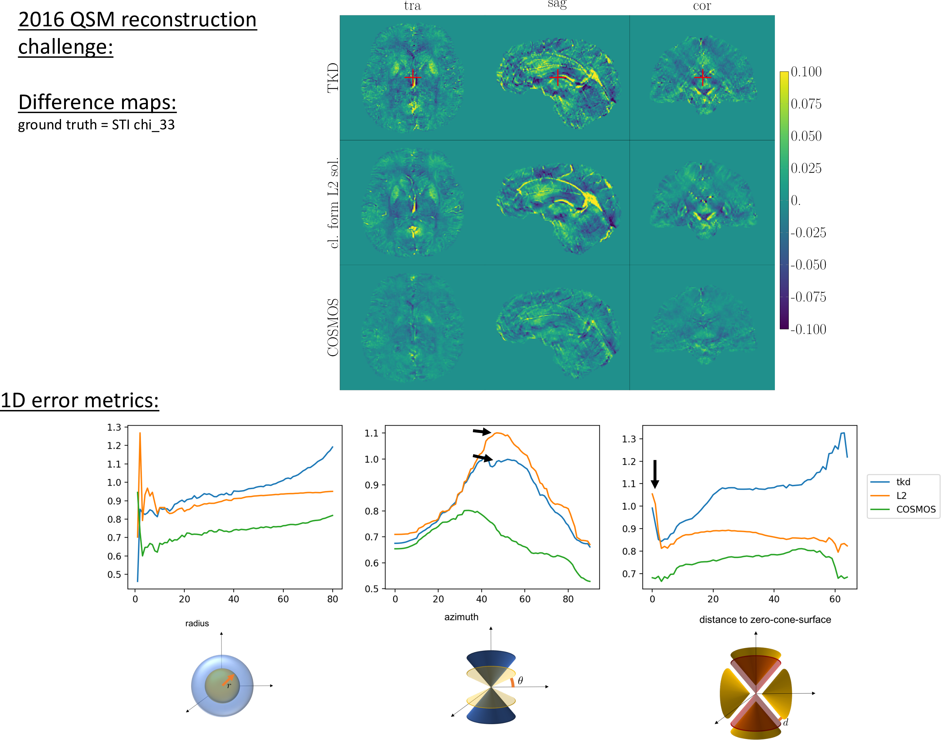
Figure 3: Comparison of one-dimensional metrics between the baseline QSM reconstructions (TKD6, L27, COSMOS8) and the reference (STI 33 9) from the 2016 QSM reconstruction challenge3. Differences on cone surfaces illustrate fundamental difference in the dipole inversion methods, e.g. the reduced error of TKD compared to L2 around the magic angle of $$$54.7^\circ$$$ due to the TKD-characteristic change of the dipole kernel in this region.
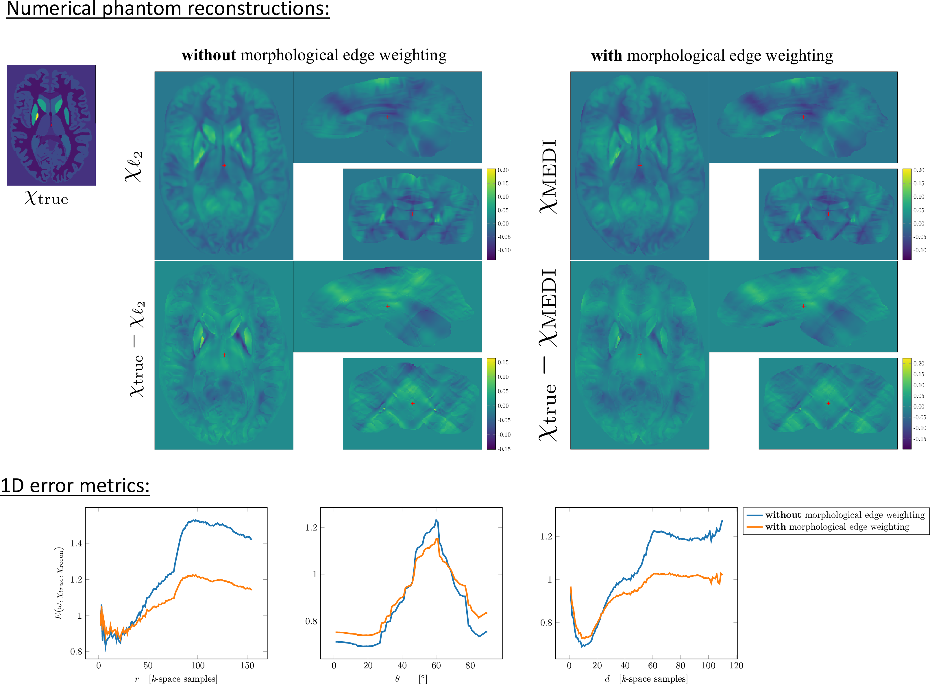
Figure 4: Computed 1D metrics for numerical brain phantom QSM to compare and understand the effect of a morphological edge weighting in the MEDI regularizer11. Edge weighting primarily reduces the error in k-space regions far from the zero cone surface and in the k-space periphery at the cost of slightly higher errors in the k-space center.
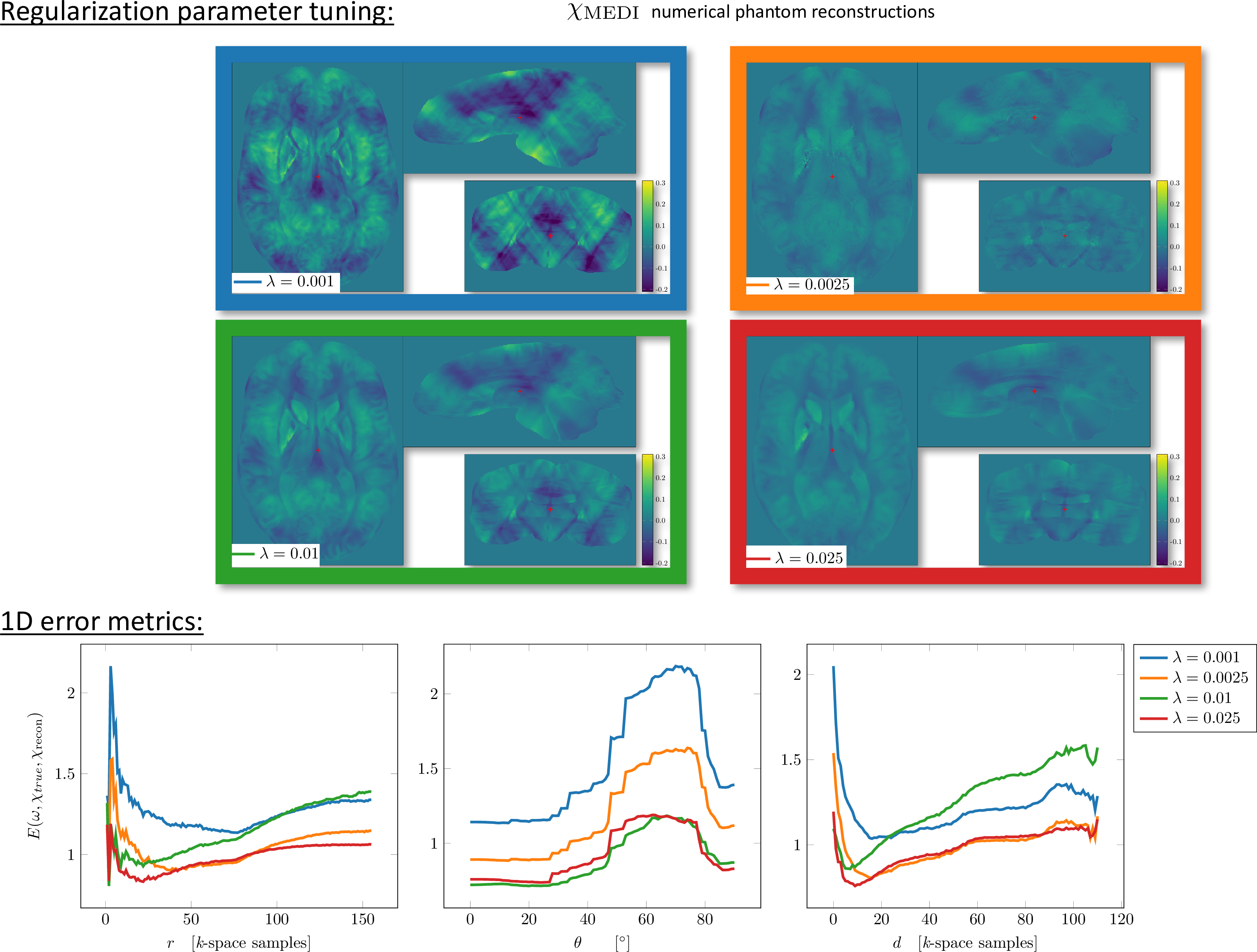
Figure 5: 1D metrics for the same numerical brain phantom for different regularization parameters demonstrating their usefulness in hyper parameter tuning. Generally stronger regularization (increased $$$\lambda$$$) reduces the errors close to the zero cone surface. The 1D metrics reveal the unfeasible regularization parameter $$$\lambda=0.01$$$ (green line), which leads to increased errors in the k-space periphery further away from the zero cone surface.The 1D metrics also distinguish the optimal regularization parameter $$$\lambda=0.025$$$ (red line) at low errors in all metrics.