0321

Deep Learning for solving ill-posed problems in Quantitative Susceptibility Mapping – What can possibly go wrong?

Pia Christine Høy¹, Kristine Storm Sørensen¹, Lasse Riis Østergaard¹, Kieran O'Brien^2,3, Markus Barth², and Steffen Bollmann²

¹Department of Health Science and Technology, Aalborg University, Aalborg, Denmark, ²Centre for Advanced Imaging, The University of Queensland, Brisbane, Australia, ³Healthcare Pty Ltd, Siemens, Brisbane, Australia

Synopsis

Quantitative susceptibility mapping (QSM) aims to solve an ill-posed field-to-source inversion to extract magnetic susceptibility of tissue. QSM algorithms based on deep convolutional neural networks have shown to produce artefact-free susceptibility maps. However, clinical scans often have a large variability, and it is unclear how a deep learning-based QSM algorithm is affected by discrepancies between the training data and clinical scans. Here we investigated the effects of different B0 orientations and noise levels of the tissue phase on the final quantitative susceptibility maps.

Introduction

Quantitative susceptibility mapping (QSM) is a post processing technique, which has shown promise with regard to quantification of iron deposits and myelination of white matter^1-4. QSM aims to construct a magnetic susceptibility map from a gradient echo MR phase image, which requires phase unwrapping, background field removal, and solving an ill-posed inverse problem^2,4,5. Recently, deep convolutional neural networks have been proposed for solving the inverse problem, and showed to produce artefact-free susceptibility maps.^6,7 However, MRI scans vary based on scanner type, field strength and scan parameters⁸ and therefore, produce different numerical inputs for neural networks. It is not clear what effect discrepancies between training data characteristics and clinical data have on the performance of deep learning QSM (DL-QSM) algorithms. Here we investigate the effect of the object orientation with respect to B0 and the impact of tissue phase noise on the performance of a deep learning QSM algorithm trained on synthetic data.

Methods

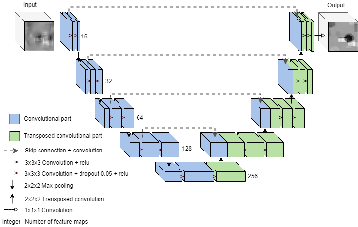
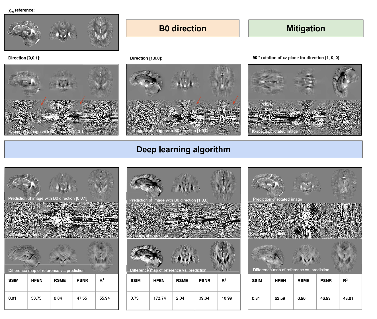
The architecture of our network is based on the U-Net⁹ and can be seen in Figure 1. This architecture has shown to be efficient at solving inverse problems in imaging¹⁰. The QSM algorithm was implemented in Python 3.6 with Tensorflow version 1.611, and trained on 100,000 synthetic examples of size 64x64x64 in 91,600 steps, with a total training time of 35 hours on a NVIDIA Tesla V100 Accelerator Unit. The three-dimensional synthetic training data was randomly extracted from a 160x160x160 image containing between 80 and 120 cubes that were randomly rotated between 0 and 180 degrees and between 80 and 120 spheres. The shape sizes varied between 10% and 40% of the image size. The susceptibility value of each shape was drawn from a uniform distribution ranging from -0.2 to 0.2 ppm. Before extraction of the training samples, the image was convolved with the unit dipole kernel. The Adam optimizer¹² with an initial learning rate of 0.001, β1 of 0.9 and β2 of 0.99 was used to update network weights, and mean squared error was used as error metric during training. Data from the 2016 reconstruction challenge¹³ was used with the χ₃₃ solution as reference. The forward image was manipulated according to the examined parameter to determine the effect on the predictions. Where applicable, a mitigation was proposed, and its effect on the performance was examined. The performance was evaluated quantitatively using the structural similarity index (SSIM), high-frequency error norm (HFEN), residual mean-squared error (RMSE), peak signal to noise ratio (PSNR) and coefficient of determination (R2), and qualitatively by visual assessment and difference maps.

Results and Discussion

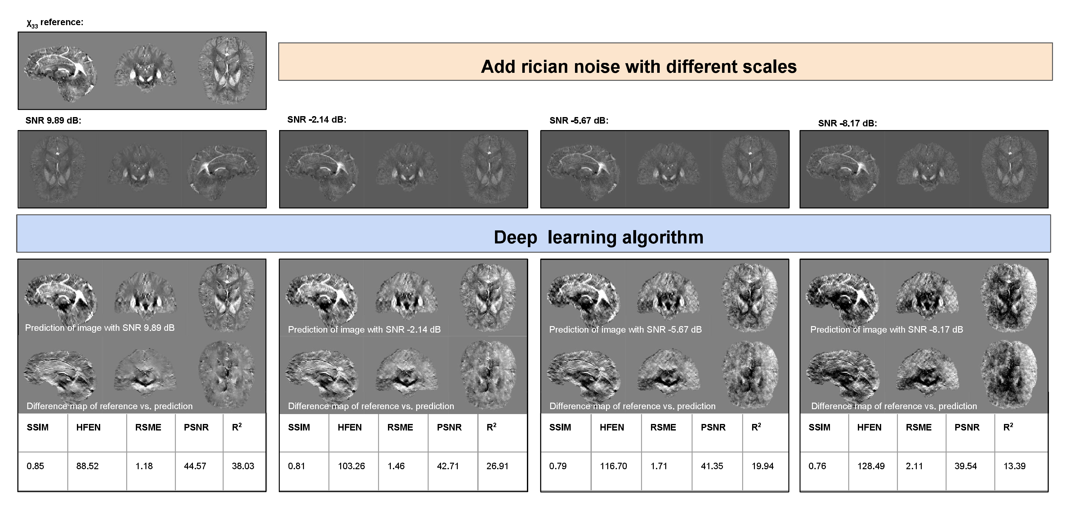
Figures 2 and 3 show the results of the investigation of the B0 direction and added noise. Since the DL-QSM algorithm was trained on a particular B0 direction ([0, 0, 1]), we hypothesised that a deviation from this direction would affect the performance. Our results show that this is the case and it can be clearly seen that the inversion completely fails when the network predicts on a non-trained direction ([1, 0, 0]). It can also be seen that the dipole kernel has an incorrect orientation in the k-space plots in Figure 2 (arrows). One mitigation to this effect was found by rotating the input before applying it to the network. After rotating the image matrix the k-space now reflects the learned dipole orientation and the dipole inversion works again. The performance of the DL-QSM algorithm decreases with increased noise level. This is reflected by a darkening particularly in the centre of the brain that becomes progressively worse as seen in Figure 3. One potential mitigation to this problem could be the addition of noise during training to make the network more robust to this influence.

Conclusion

We found that the studied DL-QSM algorithm performs best, when the dipole kernel direction of the input resembles the direction of the training data. We also found that the studied network was not robust to high levels of image noise. Future optimization should focus on more complex mitigations such as improvement of training data or application of a QSM tailored error metric during learning with the goal to increase robustness to the described parameters.

Acknowledgements

This study was supported by the facilities of the National Imaging Facility at the Centre for Advanced Imaging, the University of Queensland, as well as resources and services from the National Computer Infrastructure (NCI), supported by the Australian Government. The first two authors acknowledge funding from Aalborg University Internationalisation foundation, Otto Mønsted foundation, Knud Højgaard foundation, Danish Tennis Foundation, Nordea foundation, Marie and M. B. Richters foundation and the Oticon foundation.

References

1. Liu C, Wei H, Gong N, et al. Quantitative Susceptibility Mapping: Contrast Mechanisms and Clinical Applications. Tomography 2015; 1(1): 3-17

2. Reichenbach J. R, Schweser F, Serres B, et al. Quantitative Susceptibility Mapping: Concepts and Applications. Clin Neuroradiol. 2015; 25: 225-230

3. Wang Y, Spincemaille P, Liu Z, et al. Clinical Quantitative Susceptibility Mapping (QSM): Biometal Imaging and Its Emerging Roles in Patient Care. J. Magn. Reson. Imaging 2017; 46: 951-971

4. Haacke E. M, Liu S, Buch S, et al. Quantitative susceptibility mapping: current status and future directions. Magnetic Resonance Imaging 2015; 33: 1-25

5. Deistung A, Schweser F, Reichenbach J. R. Overview of quantitative susceptibility mapping. NMR in Biomedicine 2017; 30(4)

6. Rasmussen K. G. B, Kristensen M, Blendal R. G, et al. DeepQSM – Using Deep Learning to Solve the Dipole Inversion for MRI Susceptibility Mapping. 2018: 1-9. doi:10.1101/278036

7. Yoon J, Gong E, Chatnuntawech I, et.al. Quantitative susceptibility mapping using deep neural network: QSMnet.NeuroImage 2018; 179:199-206

8. Helmer K. G, Chou M-C, Preciado R. I, et. al. Multi-site of diffusion metric variability: effects of site, vendor, field strength, and echo time on regions-of-interest and histogram-bin analyses. Proc SPIE Int Soc Opt Eng. 2016. doi: 10.1080/10937404.2015.1051611.INHALATION

9. Ronneberger O, Fischer P and Brox T. U-Net: Convolutional Networks for Biomedical Image Segmentation. Medical Image Computing and Computer-Assisted Intervention – MICCAI 2015 234–241. doi:10.1007/978-3-319-24574-4_28

10. Jin K. H, McCann M. T, Froustey E and Unser M. Deep Convolutional Neural Network for Inverse Problems in Imaging. IEEE Trans. Image Process. 2017; 26: 4509–4522

11. Abadi M, Agarwal A, Barham P. et al. Tensorflow: Large-scale machine learning on heterogeneous distributed systems. ArXiv Prepr. ArXiv160304467 (2016).

12. Kingma D. P, Ba J. L. Adam: A Method of Stochastic Optimization. Conference Paper at ICLR 2015

13. Langkammer C, Schweser F, Shmueli K, et al. Quantitative Susceptibility Mapping: Report from the 2016 Reconstruction Challenge. Magnetic Resonance in Medicine 2018; 79: 1661–1673

Figures

Figure 1: The architecture of our network based on the U-Net ⁹. The architecture contains a convolutional and transposed convolutional part linked by skip connections. The convolutional part has convolutional layers of filter size 3x3x3 with dropout of 0.05 and relu activation function and max pooling layers. The transposed convolutional part contains convolutional layers with filter size 3x3x3 and relu activation function and transposed convolutional layers. The output layer is a convolutional layer with filter size 1x1x1. The output has the same size as the input.

Figure 2: The effect of the B0 orientation. In the top left corner the χ₃₃ reference image is shown. The reference image is convolved with dipole kernels of different directions to simulate different B0 orientations. The first two columns show slices from image and k-space representations of the input and the image, k-space, difference map and error metric values of the algorithm prediction. The third column shows that the effect of a non-trained B0 direction can be mitigated by rotating the input. The red arrows show the areas in k-space affected by the kernel.

Figure 3:Investigation of the effect of noise level of the input. In the top left corner the χ₃₃ reference image is shown. Rician noise of different levels was added to the phase tissue, and the four columns show the input image to the deep learning algorithm as well as the prediction image, difference map and error metrics for the examined SNR levels. The inversion ability of the algorithm decreases as the noise level increases, which is expressed as darkening in the centre of the brain.

Proc. Intl. Soc. Mag. Reson. Med. 27 (2019)

0321