0320
U2-Net for DEEPOLE QUASAR–A Physics-Informed Deep Convolutional Neural Network that Disentangles MRI Phase Contrast Mechanisms1Department of Computer Science and Automation, Technische Universität Ilmenau, Ilmenau, Germany, 2Buffalo Neuroimaging Analysis Center, Department of Neurology, Jacobs School of Medicine and Biomedical Sciences, Buffalo, NY, United States, 3Clinical and Translational Science Institute, University at Buffalo, Buffalo, NY, United States
Synopsis
Magnetic susceptibility is a physical property of tissues that changes with iron level and (de-)myelination. Mapping the susceptibility can help us improve our understanding of the brain and its diseases, such as multiple sclerosis and Alzheimer disease. Quantitative Susceptibility Mapping (QSM) derives the susceptibility using MRI phase data. QUASAR adds a more sophisticated physical model to QSM. Our novel U2-Net for
Introduction
MRI phase contrast is affected by various contrast mechanisms that depend on magnetic tissue properties at length scales ranging from molecular to macroscopic. The recent technique of Quantitative Susceptibility Mapping (QSM)1 aims to quantify the tissue magnetic susceptibility via the solution of the inverse physical problem of the Larmor frequency distribution $$$f$$$:
$$f=d*\chi,$$
where $$$*$$$ denotes the 3D convolution and $$$d$$$ is the unit dipole with Lorentzian sphere correction.
While being increasingly applied in clinical studies, the physical model of QSM neglects frequency contributions that are not directly related to isotropic magnetic susceptibility. In particular, the model uses the Lorentzian sphere approximation, which does not hold in anisotropic tissues as found in the brain.2 Schweser and Zivadinov3 have recently proposed an extended physical model for QSM, termed QUAntitative Susceptibility And Residual (QUASAR) mapping, which aims to separate frequency contrast $$$f_\chi$$$ adhering to the Lorentzian sphere model and frequency contrast $$$f_\rho$$$ that does not. Mapping those two contrast components according to QUASAR involves solving the highly underdetermined problem
$$f = f_\chi + f_\rho \quad (\mathrm{with\,\,} f_\chi=d*χ) \quad\quad (1)$$
with respect to both $$$\chi$$$ and $$$f_\rho$$$. While the existing approach for the QUASAR inverse problem already yields improved susceptibility maps, it requires a priori information and is only partially able to disentangle $$$f_\rho$$$ from $$$f$$$.3
To overcome this limitation, we present
- a novel neural network architecture, termed U2-Net, that reflects the structure of the physical model in Eq. (1) and
- a network training approach for DEEp learning of the Phase Origin with a Lorentzian sphere Estimation (DEEPOLE).
Methods
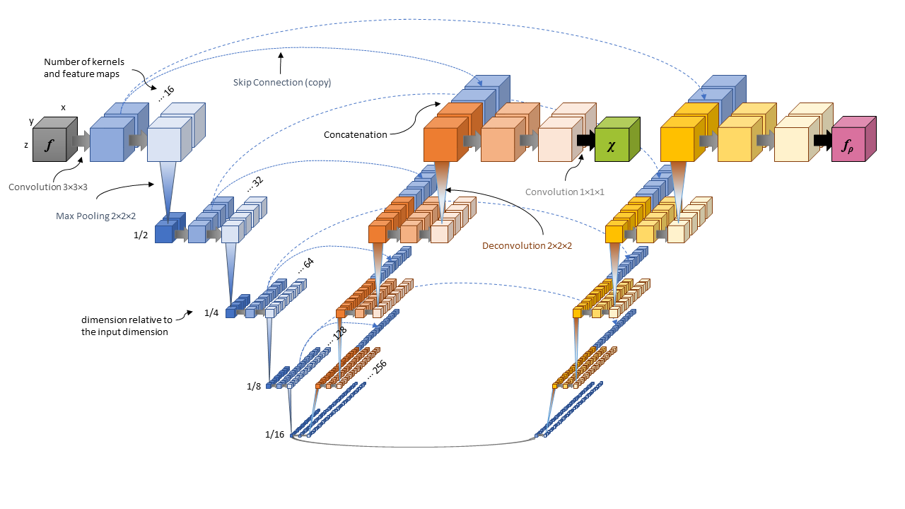
U2-Net architecture: To allow reconstructing two source patterns from one frequency map we first generalized the U-Net4 architecture to three-dimensional input and output fields and then extended it by a second expansion path (Figure 1).
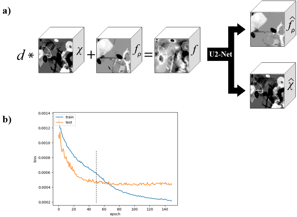
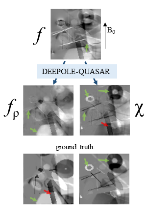
Physics-informed network training: We trained the network to simultaneously predict both volumetric scalar fields $$$f_\rho$$$ and $$$\chi$$$ from the same-sized volumetric scalar field $$$f$$$ (Figure 2a). Training was based entirely on synthetic models of $$$\chi$$$ and $$$f_\rho$$$.
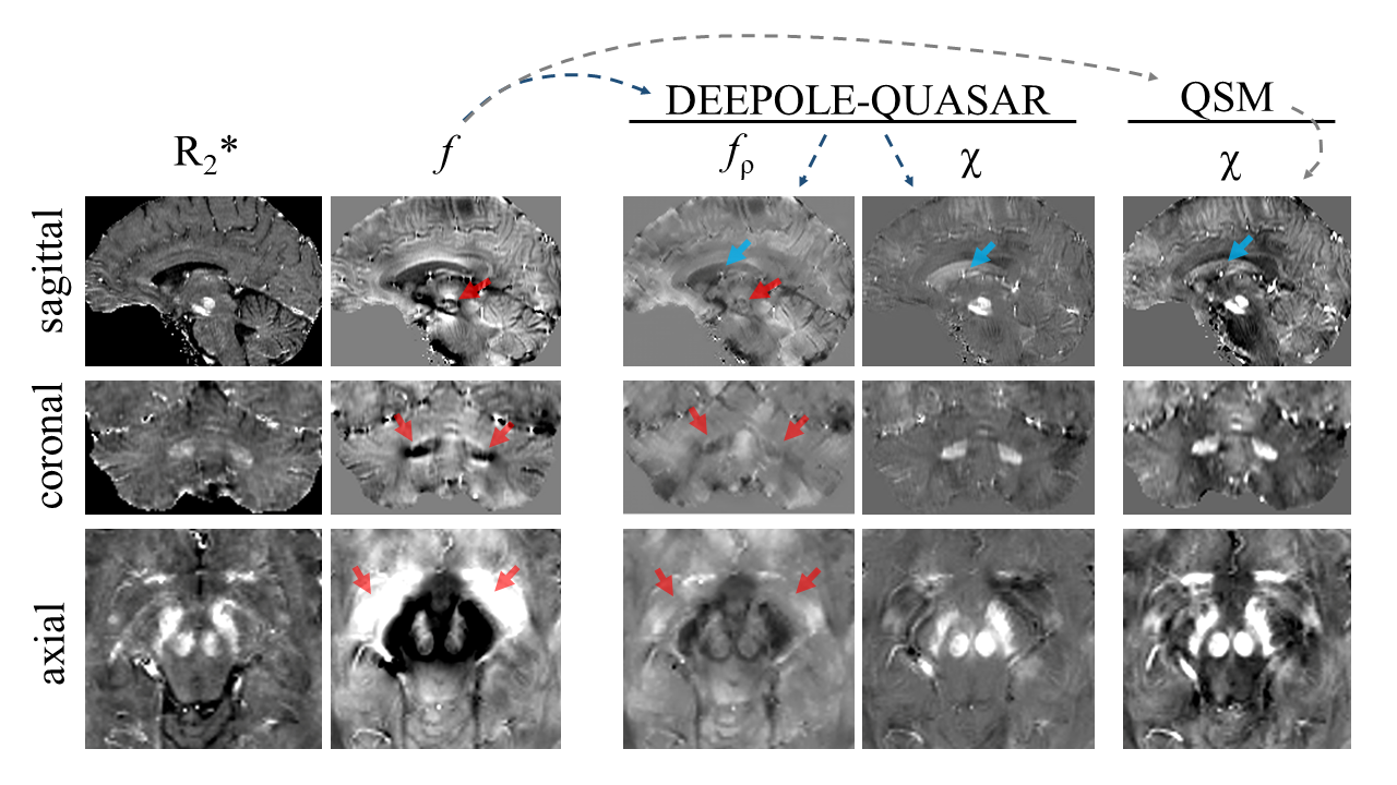
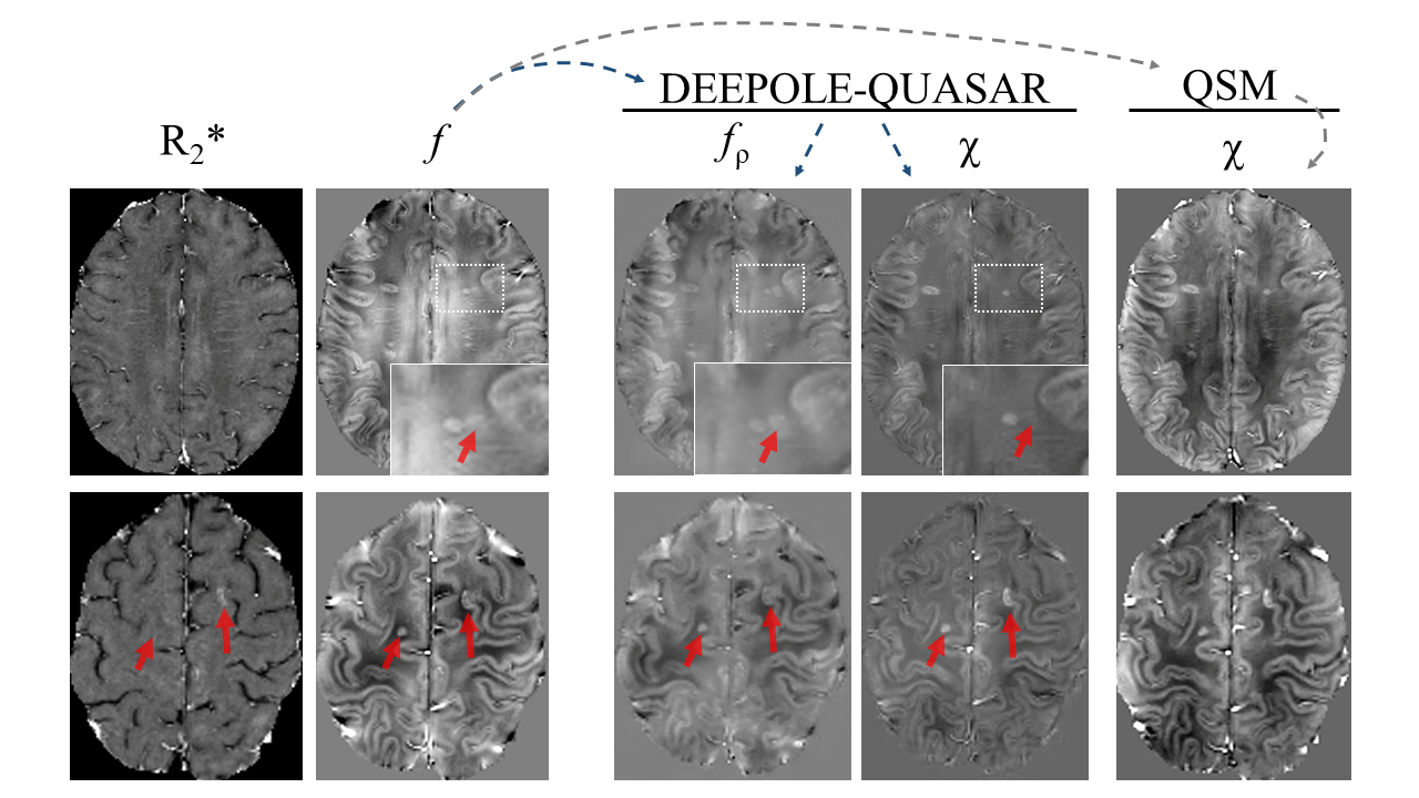
Evaluation: To evaluate the algorithm in vivo (Figures 3 and 4), we used patient data (multiple sclerosis) acquired with an axial 3D multi-echo spoiled gradient recalled echo sequence (12 echoes; 3T). We calculated $$$\chi$$$ and $$$f_\rho$$$ with the synthetically trained U2-Net and, for comparison purposes, with a conventional QSM algorithm (HEIDI).1 To evaluate the algorithm in silico, we assessed the difference between the known ground truth maps and $$$f_\rho$$$ and $$$\chi$$$ predicted from simulated $$$f$$$ (Figure 5).
Results
Figures 3 and 4 illustrate the application of the U2-Net for DEEPOLE QUASAR in vivo and compare the predicted $$$\chi$$$ with the solution obtained with the conventional QSM algorithm.1 In our examples, we could identify regions where field perturbations that were obviously caused by susceptibility alterations were correctly attributed to the susceptibility map, $$$\chi$$$, and did not appear on the $$$f_\rho$$$ map (Figure 3). The new technique also yielded more plausible susceptibility values in homogenous compartments such as the cerebrospinal fluid (CSF). DEEPOLE QUASAR discriminated lesions that showed similar contrast on the $$$f$$$ map and the conventional QSM susceptibility map (Figure 4).
Discussion
The presented algorithm bears the potential to provide information about biophysical mechanisms of frequency contrast that were not accessible until recently and that are not accounted for in the widely employed QSM model. Our experiments demonstrated the partially successful separation of the residual field component from the Lorentzian-sphere dipole component. While thorough validation of the technique is required, the $$$f_\rho$$$-contrast bears the potential for a unique and highly sensitive assessment of myelin-related pathology.
As a more general perspective, our results illustrate the ability of deep neural networks to solve underdetermined source separation problems in medical imaging (where a ground truth often is not available) by theory-guided learning from synthetic, physics-informed training data. We expect that optimized network architectures and training data generation schemes will further improve the source separation accuracy in the future.
Conclusion
Physics-informed deep convolutional neural networks are a promising tool for solving underdetermined source separation problems with a flexible incorporation of complex domain knowledge. The computational efficiency for inference (without GPU) will foster widespread application in the clinical setting.
The proposed approach sets the foundation for the quantification of biophysical tissue properties with MRI based on known physical interactions between tissue constituents, magnetic sub-cellular architecture, and the MRI signal.
Acknowledgements
Research reported in this publication was funded by the National Center for Advancing Translational Sciences of the National Institutes of Health under Award Number UL1TR001412. The content is solely the responsibility of the authors and does not necessarily represent the official views of the NIH.References
1. Schweser F, Sommer K, Deistung A, Reichenbach JR. Quantitative susceptibility mapping for investigating subtle susceptibility variations in the human brain. NeuroImage 2012;62:2083–2100 doi: 10.1016/j.neuroimage.2012.05.067.
2. He X, Yablonskiy DA. Biophysical mechanisms of phase contrast in gradient echo MRI. PNAS 2009;106:13558–13563 doi: 10.1073/pnas.0904899106.
3. Schweser F, Zivadinov R. Quantitative susceptibility mapping (QSM) with an extended physical model for MRI frequency contrast in the brain: a proof‐of‐concept of quantitative susceptibility and residual (QUASAR) mapping. NMR in Biomedicine 2018 doi: 10.1002/nbm.3999.
4. Ronneberger O, Fischer P, Brox T. U-Net: Convolutional Networks for Biomedical Image Segmentation. arXiv:1505.04597 [cs] 2015.
5. Marques JP, Bowtell R. Application of a Fourier-based method for rapid calculation of field inhomogeneity due to spatial variation of magnetic susceptibility. Concepts in Magnetic Resonance Part B: Magnetic Resonance Engineering 2005;25B:65–78 doi: 10.1002/cmr.b.20034.
6. Rasmussen KGB, Kristensen MJ, Blendal RG, et al. DeepQSM - Using Deep Learning to Solve the Dipole Inversion for MRI Susceptibility Mapping. bioRxiv 2018:278036 doi: 10.1101/278036
Figures