0241
Performance comparison of compressed sensing algorithms for accelerating T1ρ mapping of Human Brain1Center for Biomedical Imaging, Department of Radiology, New York University School of Medicine, New York, NY, United States
Synopsis
3D-T1ρ mapping sequences are useful MRI methods in various neuropathologies but its data acquisition requires long scan times. We compared the performance of 5 compressive sensing (CS) algorithms with acceleration factors (AF) up to 10. We evaluated image quality and T1ρ estimation errors as a function of AF. Six healthy volunteers were recruited and they underwent T1ρ imaging of the whole brain with full Cartesian acquisition. Assessment of image reconstruction and T1ρ estimation errors in this study show that the CS method using spatial and temporal finite differences as a regularization function performs the best for accelerating T1ρ quantification in the brain.
Introduction
3D- T1ρ mapping is a quantification technique for a number of brain applications including multiple sclerosis, Alzheimer’s and stroke[1] . Additionally, the sensitivity of T1ρ contrast to chemical exchange can potentially allow the characterization of myelin and multi-component relaxation studies[2]. However, T1ρ mapping is time consuming to acquire because of the application of multiple spin lock (TSL) pulses. Compressed sensing (CS) offers the ability to accelerate data acquisition by getting less data, below Nyquist rate[3]. CS requires iterative methods to obtain artifact free images. In this study we compared the performance of 5 CS algorithms with acceleration factors (AF) up to 10 with respect to the metrics of reconstructed image quality and T1ρ estimation errors.Methods
Six healthy volunteers (3 males, 3 females, age=28.6±5.3 years) were recruited for the study and 3D-T1ρ weighted images at varying TSL durations were acquired using a 3D Cartesian turbo-FLASH sequence with a customized T1ρ preparation module[4]. All scans were performed on a 3T clinical MRI scanner (Prisma, Siemens Healthineers, Erlangen, Germany) with a vendor supplied 20 channel receive only head-coil. The MR acquisition parameters were: TR=1500 ms, TE=2.9 ms, FOV=240mm, matrix size=256x128x64, flip angle=8°, slice thickness=2mm, spin-lock frequency=500Hz, TSL durations=[2,4,6,8,10,15,25,35,45,55] ms, total acquisition time=32 minutes.
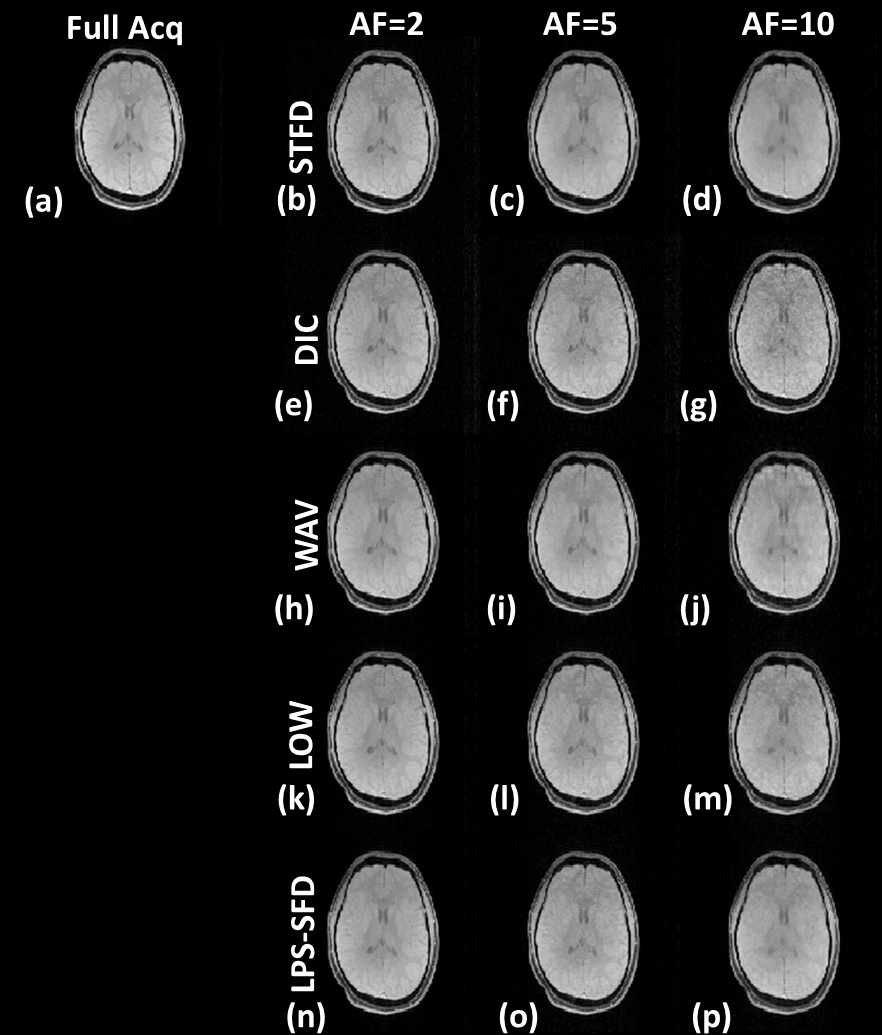
The fully sampled reconstruction served as the reference, and the resulting T1ρ maps were used to compare the performance of the CS algorithms used. The reference images were reconstructed with SENSE, with coil sensitivity maps estimated using the ESPIRiT [5]. The fully sampled dataset was retrospectively undersampled with a 2D Poisson-disk to simulate AF (AF= 2,5,10). Five different CS reconstruction models were tested with regularization functions: spatial and temporal finite differences (STFD), exponential dictionary (DIC), 3D wavelet transform (WAV), low-rank (LOW), and low-rank plus sparse model with spatial finite differences (LPS-SFD). Three techniques (STFD, DIC, WAV) used an l1-norm penalty, LOW used a nuclear norm, and the LPS-SFD used where L used nuclear norm, and the S used an l1-norm regularization penalty.
The general form of the CS reconstruction were
$$x=\arg\min_x ||y-SFCx||_2^2+λR(x).$$
where the first part is the data consistency term, with $$$y$$$ the acquired data, S is the sampling matrix, F is the Fourier transform, C represents the coil sensitivities, and $$$x$$$ is the reconstructed object. The second part is the regularization penalty where $$$R(x)=|| Tx||_1$$$ is a sparsifying penalty where T represents the transform used. For the LOW we use the nuclear norm $$$R(x)=|| x||_* $$$ and for LPS-SFD method we replace $$$R(x)$$$ by $$$λ_l||l||_*+λ_s||Ts||_1$$$, where $$$x=s+l$$$.
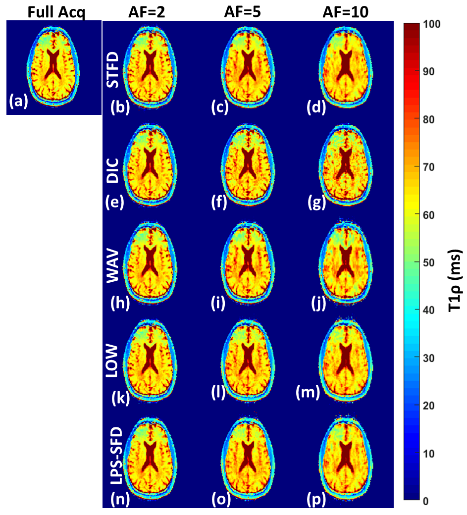
Mono-exponential T1ρ mapping for each pixel was done after CS reconstruction using the fitting model Where A is the amplitude, TSL is the spin lock durations used, T1ρ is rotating frame relaxation time and A0 is the calculated noise. Normalized root mean square error (nRMSE) was calculated to compare image quality. The T1ρ quantification error was calculated as median normalized absolute deviation (MNAD) [6].
$$S=A·e^{-TSL/T_{1ρ}}+A_0$$
Where $$$A$$$ is the amplitude, $$$TSL$$$ are the spin lock durations used, T1ρ is rotating frame relaxation time and $$$A_0$$$ is the calculated noise. Normalized root mean square error (nRMSE) was calculated to compare image quality. The T1ρ quantification error was calculated as median normalized absolute deviation (MNAD) [6].
Results
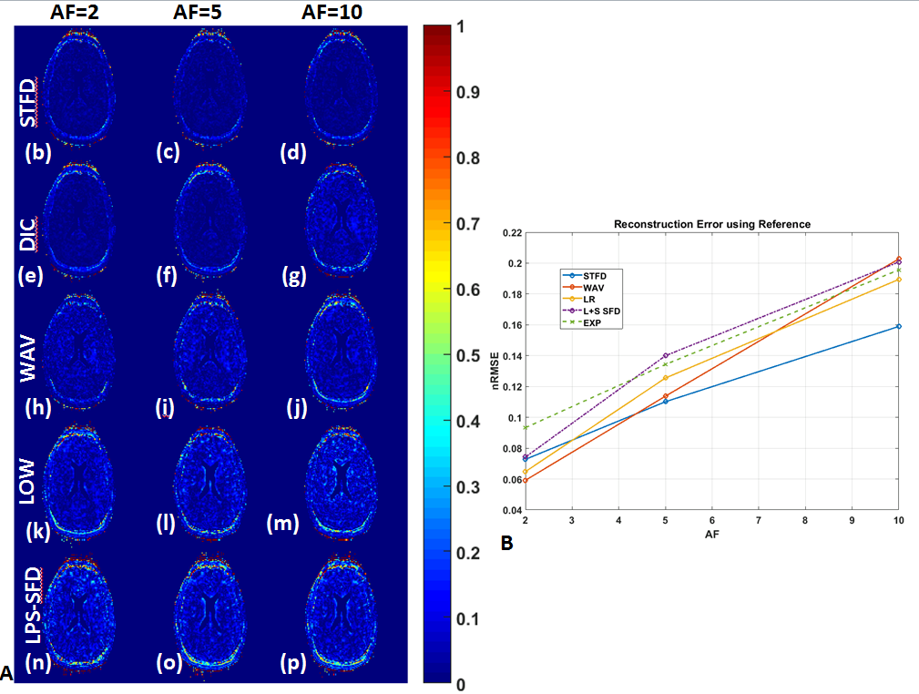
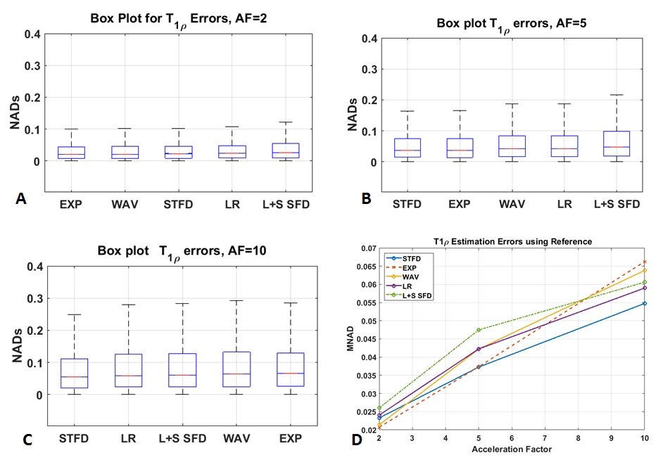
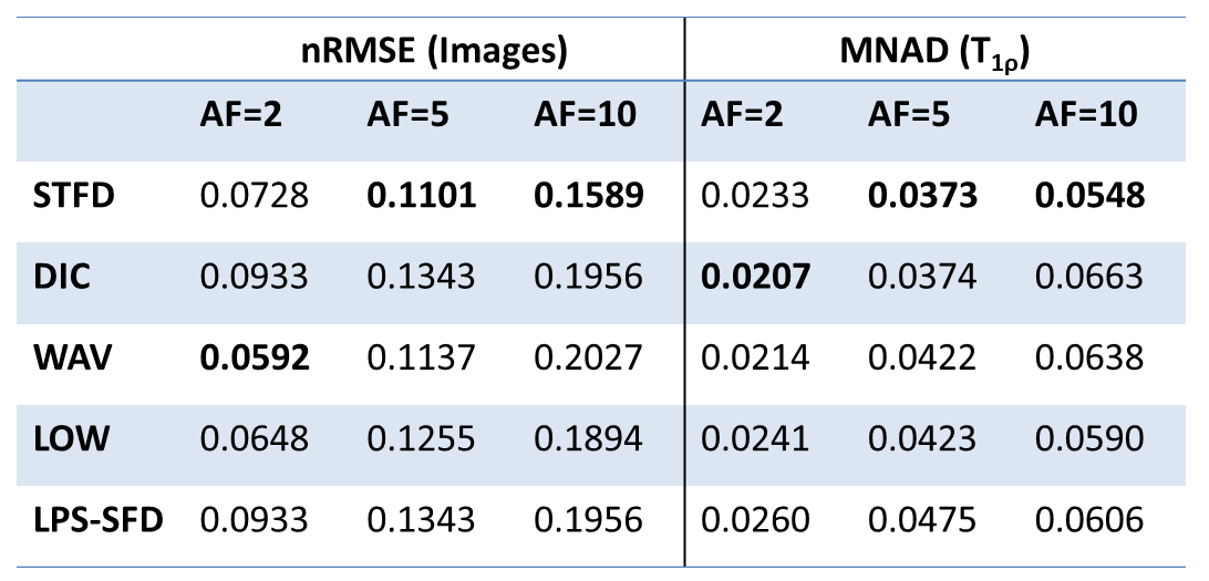
Figure 1 shows the image quality of a representative slice using the different CS algorithms used and the AF employed along with the corresponding reference image. Figure 2 shows the computed T1ρ maps using the different CS reconstruction models for a representative slice. To compare the quality of the images obtained from CS reconstruction, figure 3 shows the nRMSE error with AF. Figure 4(a-c) shows the box-plots of the NAD error in T1ρ estimation with different AF. Figure 4(d) shows MNAD error at different AF using the reference T1ρ maps. Table 1 summarizes the performance of the CS methods with reconstruction errors in the images and the T1ρ estimation errors at different AF.Discussions and Conclusions
The results in this study suggest that while at lower AF the choice of CS method is insignificant, at higher AF, the highest gain is obtained from using the STFD technique. The performance of the low rank technique is comparable but worse when compared to the STFD technique. Although L+S method is a promising approach, its performance is not better than the other techniques. The combination of first order spatial and second order temporal finite differences provides excellent performance, but the regularization parameters have to be chosen carefully to avoid being over-regularized. All images here use pre-filtered 3x3 gaussian kernel during the T1ρ fitting process. Our results are consistent with other studies in recent literature [6, 7]. The results suggest that 10X acceleration of T1ρ mapping sequences is feasible using appropriate CS reconstruction methods.Acknowledgements
This study was supported by NIH grants R01-AR060238, R01 AR067156, and R01 AR068966, and was performed under the rubric of the Center of Advanced Imaging Innovation and Research (CAI2R), a NIBIB Biomedical Technology Resource Center (NIH P41 EB017183).References
1. Gilani, I.A. and R. Sepponen, Quantitative rotating frame relaxometry methods in MRI. NMR Biomed, 2016. 29(6): p. 841-61. 2. Menon, R.G., et al., Bi-exponential 3D-T1rho mapping of whole brain at 3 T. Sci Rep, 2018. 8(1): p. 1176. 3. Lustig, M., D. Donoho, and J.M. Pauly, Sparse MRI: The application of compressed sensing for rapid MR imaging. Magn Reson Med, 2007. 58(6): p. 1182-95. 4. Sharafi, A., et al., Biexponential T1rho relaxation mapping of human knee cartilage in vivo at 3 T. NMR Biomed, 2017. 5. Uecker, M., et al., ESPIRiT--an eigenvalue approach to autocalibrating parallel MRI: where SENSE meets GRAPPA. Magn Reson Med, 2014. 71(3): p. 990-1001. 6. Zibetti, M.V.W., et al., Accelerating 3D-T1rho mapping of cartilage using compressed sensing with different sparse and low rank models. Magn Reson Med, 2018. 80(4): p. 1475-1491. 7. Bhave, S., et al., Accelerated whole-brain multi-parameter mapping using blind compressed sensing. Magn Reson Med, 2016. 75(3): p. 1175-86.Figures