0217
Dynamic Optimization of Gradient Field Performance Using a Z-Gradient Array1National Magnetic Resonance Research Center (UMRAM), Bilkent University, ANKARA, Turkey, 2Electrical and Electronic Engineering, Bilkent University, ANKARA, Turkey
Synopsis
Performance parameters of gradient coils such as size of the linearity volume, linearity error, inductance, power dissipation, gradient strength per unit current are determined at the design stage. On the contrary, array of gradient coils driven by independent amplifiers can enable optimization of this parameters. Therefore, optimal gradient performance can be realized depending on the sequence requirements and target volumes. Nine channel z-gradient array is used to optimize various performance parameters and to analyze the tradeoffs between them. Linear gradient profile generated by Z-gradient array hardware is used as readout gradient to demonstrate the feasibility of the hardware.
Introduction
Conventional gradient coils are designed to satisfy some performance parameters such as size of the linearity volume, linearity error, inductance, power dissipation, gradient strength per unit current1. As an example tradeoff, there is an inverse relation between the size of the gradient volume of interest (VOI) and PNS thresholds2. Another example is the increased efficiency of insert gradient coils compared to whole body gradient coils3 due to their smaller linearity volume.
Although different applications might require different target volumes and gradient performance metrics, performance of the conventional coils cannot be altered after manufacturing. On the contrary, gradient array coils driven by independent amplifiers can generate flexible field profiles dynamically. Previously designed 9 channel z-gradient array4 is used to increase gradient strength in selected regions by allowing more linearity error for diffusion weighted imaging5. In this study, array currents are optimized for various cost functions: (1) minimum linearity error, (2) maximum gradient strength, (3) maximum hardware slew rate, (4) current norm and (5) maximum vector B-field for VOIs with different sizes. Feasibility of gradient array’s capability to dynamically optimize the field profiles are demonstrated with simulations and phantom experiments.
Methods
Schematic illustration of the nine channel z-gradient array is provided in Fig.1. Gradient array performances are analyzed and optimized for two types of VOIs such as cylindrical and truncated ellipsoid volumes with free parameters of length (LVOI) and transverse diameter (DVOI) of VOI as shown in Fig.1a and Fig.1b respectively. Gradient linearity error, $$$\alpha$$$, is defined as $$$|G_{z}(\rho,z) )-G_{z}(0,0)|/|G_{z}(0,0)| $$$. A linear programming problem is formulated to minimize the peak $$$\alpha$$$ for variable size VOIs. To investigate the joint effect of LVOI and peak $$$ \alpha $$$ on the other gradient performances, four more optimization problems are formulated as follows:
(a) Maximization of gradient strength per unit amplifier current limit is formulated as linear programming problem.
(b) Maximization of hardware limits for slew rate per unit amplifier voltage limit is formulated as linear programming problem considering the mutual coupling between the channels6 and ignoring coil resistances.
(c) Minimization of the norm of the current vector per 1mT/m gradient strength is formulated as quadratic programming problem. Minimizing the norm of the current would also result in minimized power dissipation of the system.
(d) Minimization of the maximum amplitude of the B-field per 1mT/m gradient strength inside the cylindrical volume with a diameter of 20 cm and length of 27.5 cm is formulated as convex optimization problem.
Optimization problems are solved under the peak $$$\alpha$$$ constraint varying from 1% to 51% over given VOI and assuming identical amplifiers. Example VOI is chosen as 20 cm DSV with various truncation lengths (LVOI). (a-b) are solved using “linprog” and (c-d) are solved using “fmincon” which are built-in functions of MATLAB-2017a. Linear z-gradient profile is also optimized for minimum peak $$$\alpha$$$ over 15 cm DSV using previously measured field profiles5. Coronal image of a phantom is acquired using the optimized currents as prephaser and readout gradients of a GRE sequence in 3T scanner. Image of the same slice is also acquired using system z-gradient with the same parameters for comparison.
Results
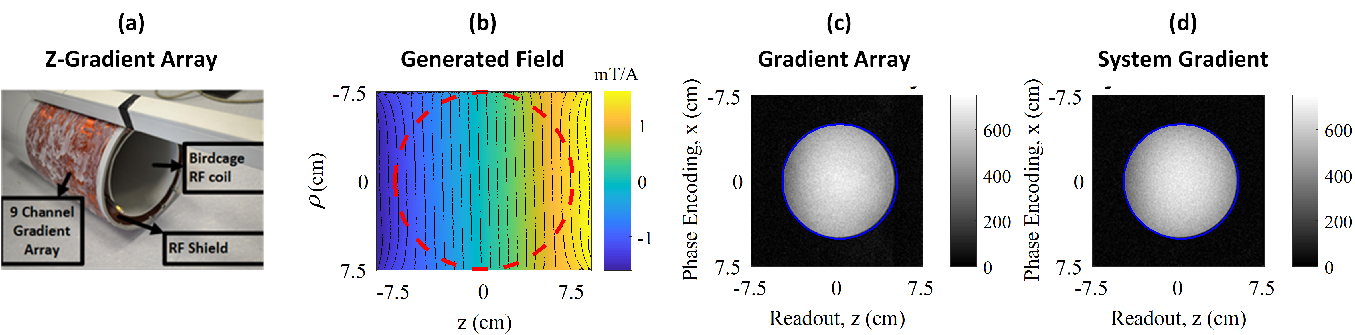
Figure 2 shows the minimum possible peak $$$\alpha$$$ for both cylindrical and ellipsoid VOIs with variable diameters and lengths. Expectedly, dimension reduction in all directions can provide lower peak $$$\alpha$$$. Optimization results of (a-d) are shown in Figure 3 which confirms that higher linearity error and/or smaller VOI can result in higher performance gradients. Figure 4 shows example magnetic field profiles generated by optimized currents for constraint pairs of (LVOI = 6 cm, 9 cm) and ($$$\alpha$$$ = 9% and 31%). Figure 4 suggest that LVOI and $$$\alpha$$$ are more effective of determining the field profile in comparison with other performance parameters. Fig.5a-b shows the experimental setup, measured optimized gradient profiles. Dimensions of the phantom image in the Fig.5c and Fig.5d confirms that gradient array system can generate fields profiles with comparable linearity error with the system gradients.Discussion and Conclusion
It is demonstrated that current of z-gradient array can be optimized for different performance parameters for a given allowed peak linearity error and size of the VOI dynamically; therefore, tradeoffs in the gradient coil design can be realized and utilized for specific goals. Continuously wounded characteristics of z-gradient array provides more flexible z-gradient field profiles because it effectively enables sampling a continuous current density as a function of z-coordinate. Finally, MRI experiments confirms the feasibility of z-gradient array hardware with a comparable performance with system gradients.Acknowledgements
No acknowledgement found.References
[1] Turner, Robert. "Gradient coil design: a review of methods." Magnetic Resonance Imaging 11.7 (1993): 903-920.
[2] Zhang, Beibei, et al. "Peripheral nerve stimulation properties of head and body gradient coils of various sizes." Magnetic Resonance in Medicine: An Official Journal of the International Society for Magnetic Resonance in Medicine 50.1 (2003): 50-58.
[3] Lee, Seung‐Kyun, et al. "Peripheral nerve stimulation characteristics of an asymmetric head‐only gradient coil compatible with a high‐channel‐count receiver array." Magnetic resonance in medicine 76.6 (2016): 1939-1950.
[4] Ertan, K., Taraghinia, S., Sadeghi, A., & Atalar, E. (2018). A z‐gradient array for simultaneous multi‐slice excitation with a single‐band RF pulse. Magnetic resonance in medicine, 80(1), 400-412.
[5] Ertan, K., Taraghinia S, Sarıtas EU, Atalar E. Local Optimization of Diffusion Encoding Gradients Using a Z-Gradient Array for Echo Time Reduction in DWI. In Proceedings of the 26th Annual Meeting of ISMRM, Paris, France, 2018. Abstract# 3194.
[6] Ertan, K., Taraghinia S, Atalar E. Driving Mutually Coupled Coils in Gradient Array Systems in Magnetic Resonance Imaging. In Proceedings of the 26th Annual Meeting of ISMRM, Paris, France, 2018. Abstract# 9133.
Figures