0213
Nonlinearity and thermal effects in gradient chains: a cascade analysis based on current and field sensing1Information Technology and Electrical Engineering, ETH Zurich, Zurich, Switzerland
Synopsis
In MRI, many gradient field imperfections are linear and time-invariant to some extend and can be well modelled by gradient impulse response functions. However, time invariance is violated by thermal effects and linearity e.g. by the gradient amplifier. To isolate sources of model violations we split the gradient chain into a cascade, consisting of eddy current compensation, amplifier and coil. Coil and amplifier responses are disentangled by extending the field measurement by current monitoring. Linearity and time-invariance violations are analyzed by performing heating experiments and varying test pulses. We show that current monitoring enables independent treatment of nonlinear distortion and thermal effects and that gradient response nonlinearities can be resolved directly.
Introduction
In MRI, the dynamic gradient fields encode spatial information and image contrast. Therefore, extremely high precision in the timing and waveform shape and knowledge about imperfections of the dynamic gradient fields are necessary. Since many imperfections, such as eddy currents, mutual coupling of gradient coils, and mechanical oscillations are linear and time-invariant to some extend they, can be well described by a matrix of gradient impulse response functions (GIRFs)1,2. However, time invariance is violated by thermal effects3 and linearity e.g. by the gradient amplifier4. Consequently, a general model would be way too complex. In this work, we follow a divide and conquer approach and split the gradient chain into a cascade, consisting of eddy current compensation (ecc), gradient amplifier and gradient coil. To disentangle coil and amplifier response we complement field measurement by current monitoring. Linearity and time-invariance violations at the different stages are analyzed by heating experiments and variation of test pulses. Finally, we show that current monitoring enables independent treatment of nonlinear distortion and thermal effects and that gradient response nonlinearities can be resolved directly.Methods
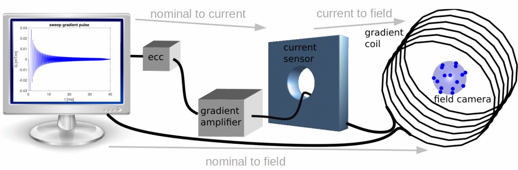
All experiments were performed with a commercial 3T imager (Achieva, Philips Healthcare). A current sensor (LEM, Switzerland) was inserted directly after the gradient amplifier on the x- and z- gradient cable (Fig. 1). Gradient field dynamics were measured as in Ref. [5] with a third-order dynamic field camera6 (Skope Magnetic Resonance Technologies). To analyze nonlinearities, gradient current and field responses of frequency swept pulses (0-30kHz) of variable duration (40/60/80/100ms), slew rate limitation (80 to 200mT/m/s) or amplitude limitation (20/30mT/m) were measured. Thereto, four partial measurements (20ms, 50ms, 60ms, 70ms) were concatenated to a single 200ms readout and the transfer functions were calculated as described in [1]. The nonlinearities were isolated, by calculating the transfer functions from scanner input (nominal) to current and from current to gradient field (Fig. 1). Multiplying these transfer functions results in the nominal to gradient field transfer function (GIRF).
To characterize thermal effects, the system was heated by playing out scans as in Ref. [7].
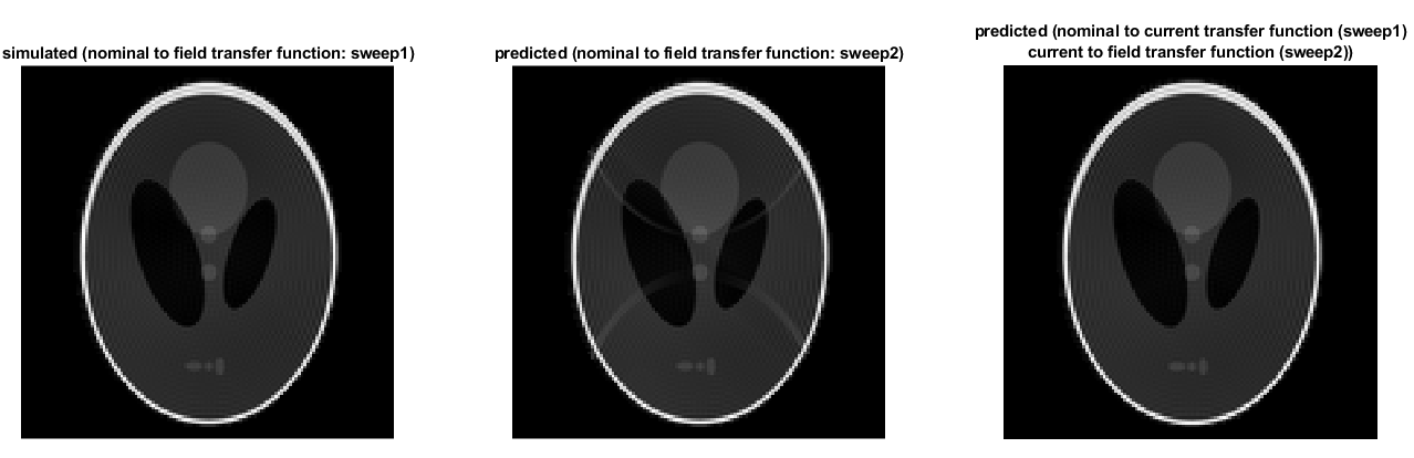
The scale of gradient response errors at the image level is assessed by simulating EPI readouts (resolution=2mm, FOV=256mm, duration=70ms) based on a k-space trajectory obtained by using the nominal to current transfer function of a 40ms sweep (sweep1). At first, the image reconstruction was performed using k-space trajectories calculated by applying the nominal to gradient transfer function of a different sweep (80ms), sweep2. This was compared to a second image reconstruction based on trajectories using the nominal to current transfer function of sweep1 (corresponding to the current measurement) and the current to field transfer function of sweep2. This simulates the effect of an image reconstruction based on concurrent current measurement.
Results and Discussion
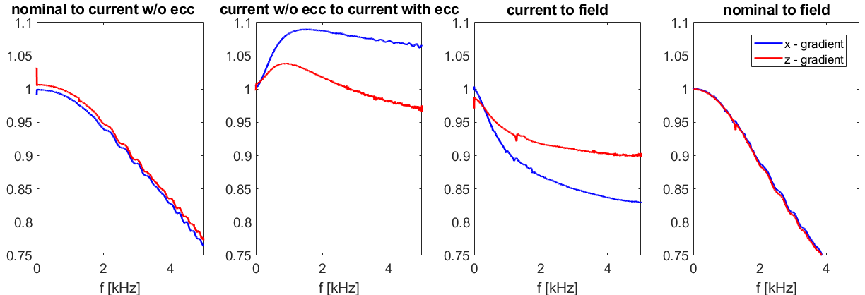
In Figure 2 the four transfer functions measured with x- and z-gradient sweep pulses are shown. It can be seen, that there are strong eddy currents which are very well compensated with the ecc. Sources for such strong eddy currents are, besides the cryostat, the (passive) x-, y- and z- gradient coils8.
The transfer functions of different x-gradient sweep pulses are shown in Figure 3a). As can be seen, nonlinear distortion only happens between scanner input and current sensor.
In Figure 3b), the current to field transfer functions vary with temperature. The nominal to current transfer function is not affected by temperature. This means, either the amplifier feedback corrects very well for the temperature dependent current variations or the heated hardware causes no change in current.
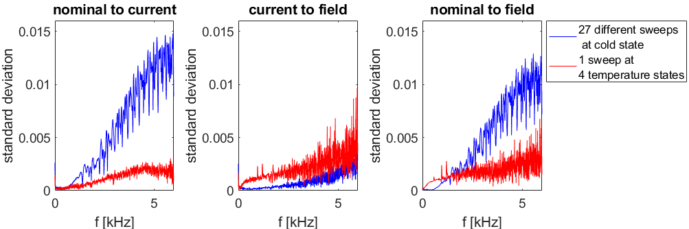
Figure 4 compares the standard deviation of the transfer functions of one sweep pulse measured at different temperatures to the standard deviation of the transfer functions of varying sweep pulses at one temperature.
Figures 3 and 4 illustrate, that the nonlinearities affect only the nominal to current transfer function and temperature only the current to field transfer function. Consequently they seem to be independent and the temperature can be treated with a thermal model7,9 of the current to field transfer function and nonlinearities can be eliminated by measuring the current.
In Figure 5, the extent of nonlinearities on image level is demonstrated in imaging simulations. Using the conventional transfer function model (GIRF) for reconstruction yields ghosting artefacts (middle), whereas the nonlinearity corrected one doesn’t (right).
Conclusions and Outlook
In this investigation, thermal and nonlinear effects have been found to hardly interact, suggesting that they can be treated independently to a large degree. Most nonlinearity occurs before the coil and can be eliminated using concurrent current monitoring or sequence-wise iterative pre-emphasis filter establishing. Thermal effects are due to coil hardware dynamics and can be addressed by thermal modelling7,9. Using combined current measurements and thermal modelling promises almost perfect trajectory prediction.Acknowledgements
No acknowledgement found.References
[1] S. J. Vannesjo, M. Haeberlin, L. Kasper, M. Pavan, B. J. Wilm, C. Barmet, and K. P. Pruessmann, “Gradient system characterization by impulse response measurements with a dynamic field camera,” Magn. Reson. Med, vol. 69, no. 2, pp. 583–593, 2013.
[2] Addy NO, Wu HH, Nishimura DG. Simple Method for MR Gradient System Characterization. In Proceedings of the 17th Annual Meeting of ISMRM, Honolulu, Hawaii, USA, 2009. p. 3068.
[3] J. Busch, S. J. Vannesjo, C. Barmet, K. P. Pruessmann, and S. Kozerke, “Analysis of temperature dependence of background phase errors in phase-contrast cardiovascular magnetic resonance,” J Cardiovasc Magn Reson, vol. 16, p. 97, 2014.
[4] S M Cox and B H Candy Class-D audio amplifiers with negative feedback. SIAM Journal on Applied Mathematics 66 (2005) 468-488.
[5] S. J. Vannesjo, B. E. Dietrich, M. Pavan, D. O. Brunner, B. J. Wilm, C. Barmet, and K. P. Pruessmann, “Field camera measurements of gradient and shim impulse responses using frequency sweeps”, Magn. Reson. Med, vol. 72, no. 2, pp. 570–583, 2014.
[6] B. E. Dietrich, D. O. Brunner, B. J. Wilm, C. Barmet, S. Gross, L. Kasper, M. Haeberlin, T. Schmid, S. J. Vannesjo, and K. P. Pruessmann, “A field camera for MR sequence monitoring and system analysis,” Magn. Reson. Med, vol. 75, no. 4, pp. 1831–1840, DOI: 10.1002/mrm.25770, 2016.
[7] J. Nussbaum , B. J. Wilm , B. E. Dietrich , and K. P. Pruessmann, „Improved thermal modelling and prediction of gradient response using sensor placement guided by infrared photography” in Proc Int Soc Magn Reson Med Sci Meet Exhib, 2018, p. 4210.
[8] Tang, Fangfang. Gradient coil design and intra-coil eddy currents in MRI systems. PhD Thesis, School of Information Technology and Electrical Engineering, The University of Queensland. 2016.
[9] B. E. Dietrich, J. Nussbaum, B. J. Wilm, J. Reber and K. P. Pruessmann, “Thermal Variation and Temperature- Based Prediction of Gradient Response” in Proc Int Soc Magn Reson Med Sci Meet Exhib, 2017, p. 0079.
Figures
a) Top: measurements of different frequency swept pulses of the x–gradient. Bottom: standard deviation of the measured transfer functions: the nominal to current transfer function varies for different input pulses. This reveals nonlinear effects between scanner input and current sensor.
b)
Top: Transfer function
measurements after heating the gradient coil by playing out different system
heating scan sequences. Only one specific sweep pulse is used. Bottom: standard
deviation of the transfer functions at different temperatures. It can be seen
that the current to field transfer function is highly affected by temperature
changes.