0194
Deep residual learning of radial under sampling artefacts for real-time MR image guidance during radiotherapy1Radiotherapy, University Medical Center Utrecht, Utrecht, Netherlands, 2MR Code B.V., Zaltbommel, Netherlands, 3Biomedical Engineering, University of Technology Eindhoven, Eindhoven, Netherlands, 4Medical Natural Sciences, VU Amsterdam, Amsterdam, Netherlands
Synopsis
MRI-guided radiotherapy using hybrid MR-Linac systems, requires high spatiotemporal resolution MR images to guide the radiation beam in real time. Here, we investigate the concept of deep residual learning of radial undersampling artifacts to decrease acquisition time and minimize extra reconstruction time by using the fast forward evaluation of the network. Within 8-10 milliseconds most streaking artifacts were removed for undersampling rates between R=4 and R=32 in the abdomen and brain, facilitating real-time tracking for MR-guided radiotherapy.
Purpose
MRI-guided radiotherapy using hybrid MR-linac systems opens up the opportunity to acquire MR data just before and during treatment to guide the treatment beam for highly mobile abdominothoracic tumors1. Ideally, 3D volumes are acquired and reconstructed in real time to fully account for all motion and adapt the treatment through tracking and plan optimization. Unfortunately, MR imaging is an inherently slow imaging modality. A simple method to reduce acquisition times is to acquire less data, at the cost of undersampling artifacts in the reconstructed images. These artifacts can be significantly reduced using iterative reconstructions, such as compressed sensing, but these are time-consuming and therefore not suitable for real-time processes. Here, we use deep learning2,3 to shift the time-consuming processing steps prior to treatment to enable real-time undersampling artifact removal. The goal was to determine the maximum undersampling rates to enable real-time tracking.Methods
Data acquisition: Eight in vivo data sets (four brain, four abdomen) were acquired on a 1.5T MRI-RT scanner (Ingenia, Philips, Best, the Netherlands). Fully sampled radial acquisitions were acquired using a multi-slice 2D (M2D) balanced steady-state free precession (bSSFP) cine sequence (TR/TE = 4.6/2.3ms, FA = 40o, resolution = 1.0x1.0x5.0mm3, FOV = 256x256x100mm3, number of dynamics = 20). Additionally, two extra 3D golden-angle stack-of-stars bSSFP data sets with fat suppression were acquired for the abdominal volunteers (TR/TE = 2.9/1.45ms, FA = 40o, resolution = 1.7x1.7x4.0mm3, FOV = 377x377x256mm3, acquisition time = 3m14s) for prospective undersampling.
Reconstruction: Complex data were retrospectively undersampled in k-space by factors R=4 to R=32 and reconstructed using the non-uniform FFT4. Data was divided into training (80%) and test (20%) sets and normalized per scan. Data of one volunteer were used for testing for the brain, abdomen M2D, and abdomen 3D data. 2D slices were the input for the network. Data augmentation in the form of flipping and rotating was used to increase the size and variability within the training sets.
Deep learning: A U-net was used for residual learning; the undersampling artifacts were estimated from the undersampled images, which were subsequently subtracted from the undersampled images to obtain artifact-free images, since the topology of streaking artifacts is simpler (to learn) than the artifact-free images3. A relatively shallow U-net was implemented in Keras using a TensorFlow backend (see Figure 1)3. Additional features were a hyperbolic tangent (Tanh) activation function, Adam optimizer with learning rate decay of 0.0001 and training batches of 8. Training and testing was performed on a 16Gb Nvidia Tesla P100 GPU.
Evaluation: Both the predicted artifact images and calculated artifact-free images were compared with ground-truth images using the structural similarity (SSIM)5 and information content weighted multi-scale SSIM (IW-SSIM)6. Additionally, the Fourier radial error spectrum plot (ESP)7 was calculated between calculated artifact-free and ground truth images to get insight into the error at different spatial frequencies. Lastly, deformable vector fields (DVFs)8 were calculated through non-rigid registration between ground truth images at the same location and compared to DVFs calculated after registering the networks’ output.
Results and discussion
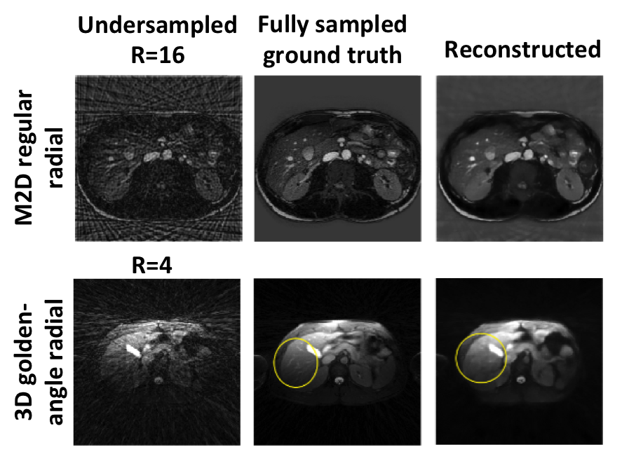
Training took on average 25 hours per data set. Forward evaluation was only 8-10 milliseconds per image. Figures 2 and 3 give examples for the brain images for R=8 (figure 2), R=16, 24 and 32 (figure 3), showing good image quality, but increased blurring and decreased visualization of details for higher undersampling levels (SSIM = 0.867, 0.842, 0.820, IW-SSIM = 0.999, 0.998, 0.998 for R=16, 24, and 32 respectively). Figure 4 shows results for M2D (R=16) and 3D golden-angle radial data (R=4), which were the highest acceleration factors with good image quality (SSIM>0.8). It is hypothesized that the lower R for the golden-angle data is due to motion and the prospective nature of undersampling golden-angle data. Figure 5 shows an ESP example for the three different datasets, displaying fewer errors after artifact removal. Lastly, the DVFs indicated that the difference in motion determined on the deep-learned images is small (0.83±0.75mm, 1.28±1.44mm for M2D and 3D golden-angle, respectively) relative to the ground-truth DVF.Conclusion
Radial undersampling artifacts were resolved in 8-10 milliseconds using a deep-learned network. Using the quantitative measures, it was determined that R=32, R=16, and R=4 were the maximum acceleration factors for the brain, M2D abdomen, and 3D abdominal data, respectively. Although this approach requires the reconstruction of images, the fast execution and reduction in acquisition time outweighs this disadvantage, enabling real-time image guidance. Next steps will focus on direct learning from k-space, validation in a prospective study, and setting up a database of complex data for deep learning approaches in MRI-guided radiotherapy.Acknowledgements
This work is part of the research programme HTSM project number 15354, which is partly financed by the Netherlands Organisation for Scientific Research (NWO).References
[1] Raaymakers BW, et al. First patients treated with a 1.5T MRI-Linac: clinical proof of concept of a high-precision, high-field MRI guided radiotherapy treatment. PMB2017;62:L41
[2] Lee D, et al. Deep residual learning for compressed sensing MRI, IEEE ISBI2017:15-18
[3] Han Y, et al. Deep learning with domain adaptation for accelerated projection reconstruction MR, MRM2018;80:1189-1205
[4] Fessler JA, et al. Nonuniform fast fourier transforms using min-max interpolation, IEEE T-SP, 2003;51:560-574
[5] Wang, et al. Image quality assessment: from error visibility to structural similarity, IEEE TIP, 2004;13:600-612
[6] Wang Z, et al. Information content weighting for perceptual image quality assessment, IEEE TIP,2011;20:1185-1198
[7] Kim, TH, et al. The fourier radial error spectrum plot: a more nuanced quantitative evaluation of image reconstruction quality, 15thIEEE ISBI, 2018:61-64
[8] Zachiu C, et al. An improved optical flow tracking technique for real-time MR-guided beam therapies in moving organs, PMB, 2015;60:9003-9010
Figures