0152
150× acceleration of myelin water imaging data analysis by a neural network1Physics & Astronomy, University of British Columbia, Vancouver, BC, Canada, 2International Collaboration on Repair Discoveries, Vancouver, BC, Canada, 3Radiology, University of British Columbia, Vancouver, BC, Canada, 4Biomedical Engineering, University of British Columbia, Vancouver, BC, Canada, 5Kinesiology, University of British Columbia, Vancouver, BC, Canada, 6Pathology & Laboratory Medicine, University of British Columbia, Vancouver, BC, Canada
Synopsis
In-vivo information of myelin content is desirable for studying many brain diseases and injuries which damage myelin. Myelin water imaging (MWI) is a validated and quantitative MR method to myelin. However, the data post-processing of MWI is mathematically complex and computationally demanding. The analysis typically takes several hours for a whole brain analysis, which limits its clinical applications. Our objective was to train a neural network as an alternative method for the MWI data analysis. We found this novel approach can accelerate MWI data analysis by over 150 times.
Introduction
Myelin water imaging (MWI) has been extensively applied in the research of many myelin-related diseases such as multiple sclerosis.1 MWI uses multi-echo sequences2-4 to characterize multi-exponential T2 decays. A common analysis approach is for voxel-wise decay curves to be fitted by a regularized non-negative least squares (NNLS) algorithm with stimulated echo correction to produce a T2 distribution5 of water components. The ratio of myelin water signal to the total signal is the myelin water fraction (MWF), a histologically validated measure of myelin.6
Despite reductions in scan time to under 8 minutes7, for multiple sclerosis, and other demyelinating diseases, clinical use of MWI has not yet been realized. The computational time required for whole brain data analysis using NNLS typically takes several hours, which is unacceptable in clinical settings. In addition, regularized NNLS fitting with stimulated echo correction is mathematically complex, making it difficult to implement for new users. To resolve these issues, we proposed to train a deep learning neural network to calculate MWF, using the latest NNLS algorithm to produce the ground truth training data, so that the neural network that can (1) produce faster voxel-wise MWF calculations on new data and (2) be easier to implement.
Methods
Data acquisition: MWI data (3D gradient spin echo (GRASE), 32-echo, TE/TR=10/1000ms, slices=40, 232x192 matrix, reconstruction resolution=1x1x2.5mm3, slice oversampling factor 1.3, acquisition time 14.4min) from 6 healthy brains were collected at 3T (Philips Achieva).4
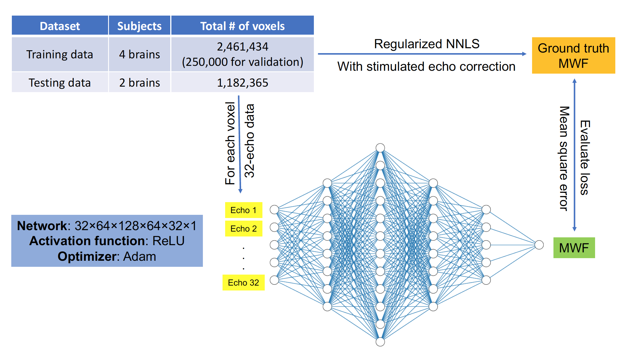
Training and testing datasets: 32-echo decay data of each voxel from the 6 brains were extracted as input datasets. 2,461,434 voxels from four brains were used for training (randomly shuffled), of which 250,000 voxels were used as a validation set to determine the stopping criterion. The remaining two brains were used for testing (1,182,365 voxels).
Ground truth: Voxel-wise 32-echo decay data were analyzed by regularized NNLS with stimulated echo correction (in-house MATLAB software)5 to compute MWF as the ground truth label for each voxel.
Neural network model: A network with 6 fully connected layers (32×64×128×64×32×1, activation function: ReLU, optimizer: Adam, loss: mean square error) was constructed using Keras with Tensorflow8 backend to take the 32-echo data as input and predict MWF at the output layer (Figure 1 depicts workflow). The training was stopped when the accuracy on the validation set did not improve further.
Neural network model evaluation: The trained model was applied to the two testing brains and the resulting MWF were compared voxel-wise with the ground truth for whole brain and 6 regions of interest (ROI) (whole gray matter, whole white matter, corpus callosum, corticospinal tract, forceps major, forceps minor). ROIs were chosen from JHU atlas9 and registered to GRASE-space. Absolute and relative differences, correlations (R-square, p-value) between predictions and ground truth, and mean absolute error (MAE) were assessed. Processing times of the neural network model and NNLS for whole brain analysis were recorded (CPU: Intel(R) Core(TM) i7-5930K @ 3.50GHz).
Results
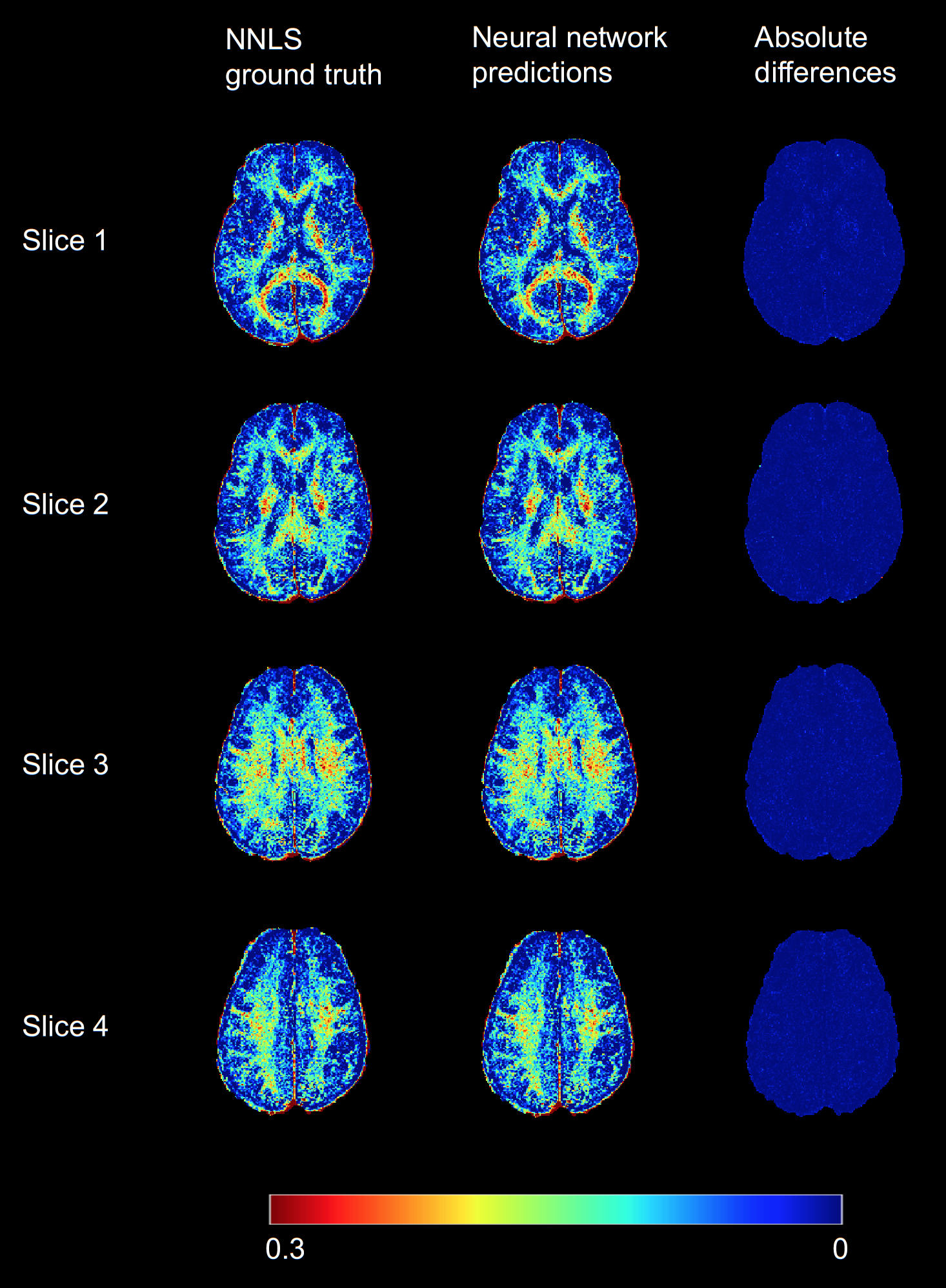
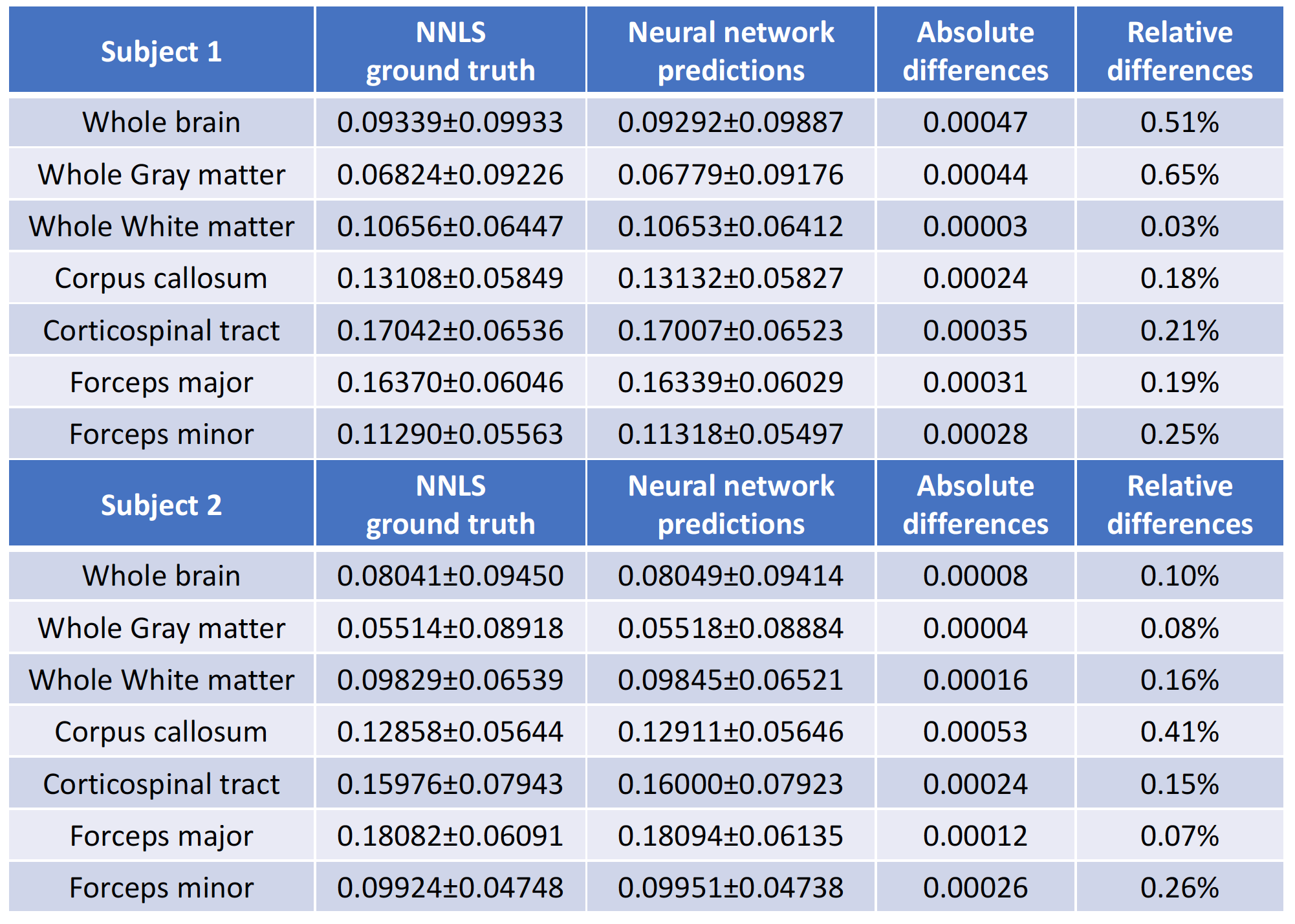
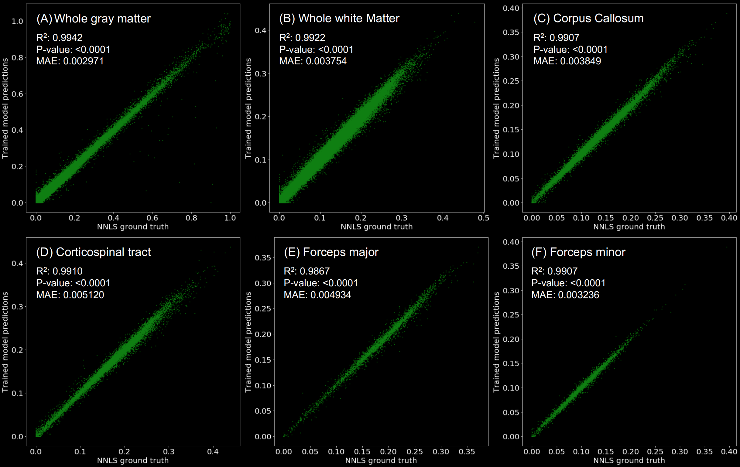
Figure 2 shows excellent visual correspondence between MWF maps from the neural network model and NNLS. Neural network model MWF predictions and the ground truth for the two testing subjects are summarized in Table 1. Neural network voxel-wise MWF correlated strongly with NNLS MWF within six different ROIs (average R2=0.9909, p<0.00001, Figure 3). The processing time for whole brain analysis was 35 seconds for the neural network model and 1.5 hours for NNLS.Discussion
No visual differences between the neural network model and NNLS MWF maps were observed, and no obvious regional biases were found (Figure 2). Quantitively, almost all voxels within each ROI exhibited excellent agreement between neural network and NNLS (Figure 3). Absolute differences of mean MWF can only be found after four decimal places and the relative differences were <1% for all ROIs, and <0.5% for white matter regions (Table 1). The extremely low error of the neural network model demonstrates that it is capable of calculating virtually the same MWF maps as NNLS for the whole brain. Most importantly, the processing speed of the neural network model was more than 150 times faster than that of the NNLS algorithm. In addition, the neural network model is much easier to implement by using many open-source machine learning frameworks such as Tensorflow.7Conclusion
We have shown that MWI data processing time can be dramatically reduced from hours to less than one minute (over 150× acceleration) without degrading the analysis results by using a trained neural network which can be easily implemented. These improvements would potentially make MWI clinically feasible. Training on a larger data set and testing on patient populations is an important next step.Acknowledgements
We thank the study participants and the excellent MRI technologists at the UBC MRI Research Centre. Funding support was provided by the Multiple Sclerosis Society of Canada, Natural Sciences and Engineering Research Council Discovery Grant.References
1. Kolind S, Seddigh A, Combes A, et al. Brain and cord myelin water imaging: A progressive multiple sclerosis biomarker. Neuroimage Clin. 2015;9:574-580.
2. Whittall KP, MacKay AL. Quantitative interpretation of NMR relaxation data. Journal of Magnetic Resonance (1969). 1989;84(1):134-152.
3. MacKay A, Whittall K, Adler J, Li D, Paty D, Graeb D. In vivo visualization of myelin water in brain by magnetic resonance. Magn Reson Med. 1994;31(6):673-677.
4. Prasloski T, Rauscher A, MacKay AL, et al. Rapid whole cerebrum myelin water imaging using a 3D GRASE sequence. Neuroimage. 2012;63(1):533-539.
5. Prasloski T, Mädler B, Xiang Q, MacKay A, Jones C. Applications of stimulated echo correction to multicomponent T2 analysis. Magnetic Resonance in Medicine. 2012;67(6):1803-1814.
6. Laule C, Leung E, Li DK, et al. Myelin water imaging in multiple sclerosis: Quantitative correlations with histopathology. Mult Scler. 2006;12(6):747-753.
7. Zhang J, Vavasour I, Kolind S, Baumeister B, Rauscher A, MacKay AL. Advanced myelin water imaging techniques for rapid data acquisition and long T2 component measurements. Proc. Int. Soc. Mag. Reson. Med. 2015;23.
8. Abadi M, Barham P, Chen J, et al. Tensorflow: a system for large-scale machine learning. In OSDI. 2016;16:265-283.
9. Mori, S., Wakana, S., Zijl, P. C. M. van & Nagae-Poetscher, L. M. MRI Atlas of Human White Matter. (Elsevier, 2005).
Figures