Introduction

Chemical exchange saturation transfer (CEST) is a novel contrast mechanism in MRI¹. However, a successful translation of CEST into clinic might be hampered by its time-consuming acquisition. With the successful application of compressed sensing (CS) theory in MRI^2,3, several CS techniques have been applied to accelerate CEST^4-6. However, CS based methods are computational expensive. Deep learning is the new frontier for MRI reconstruction^7,8, and deep convolutional network⁹ had been tested with CEST¹⁰. As recent advancement, a convolutional recurrent neural network (CRNN¹¹) was introduced, which learns the spatial-temporal dependencies in dynamic MRI, and has shown high quality reconstruction in single coil heart imaging¹¹. Here, we extended the framework combining multi-coil data into training network to accelerate parallel CEST-MRI. Using retrospectively sub-sampled in-vivo CEST-MRI data, we demonstrate that the reconstruction quality of the proposed learning framework is much better than the traditional dynamic compressed sensing method³, while the reconstruction time is about one hundred times shorter.

Theory and Methods

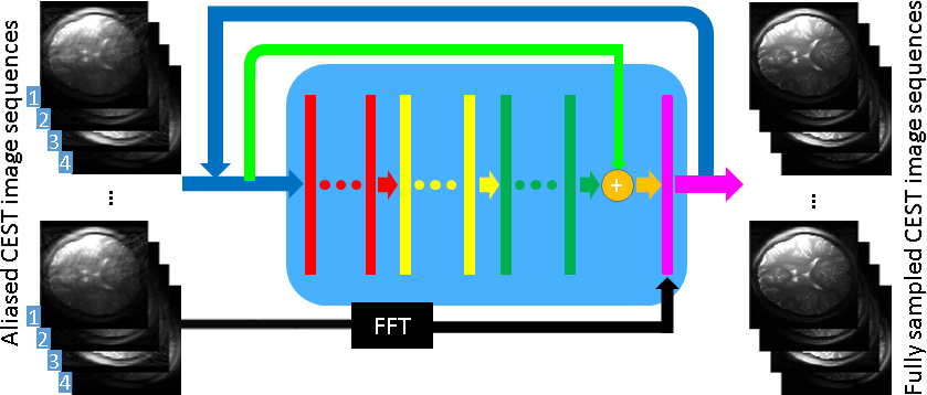
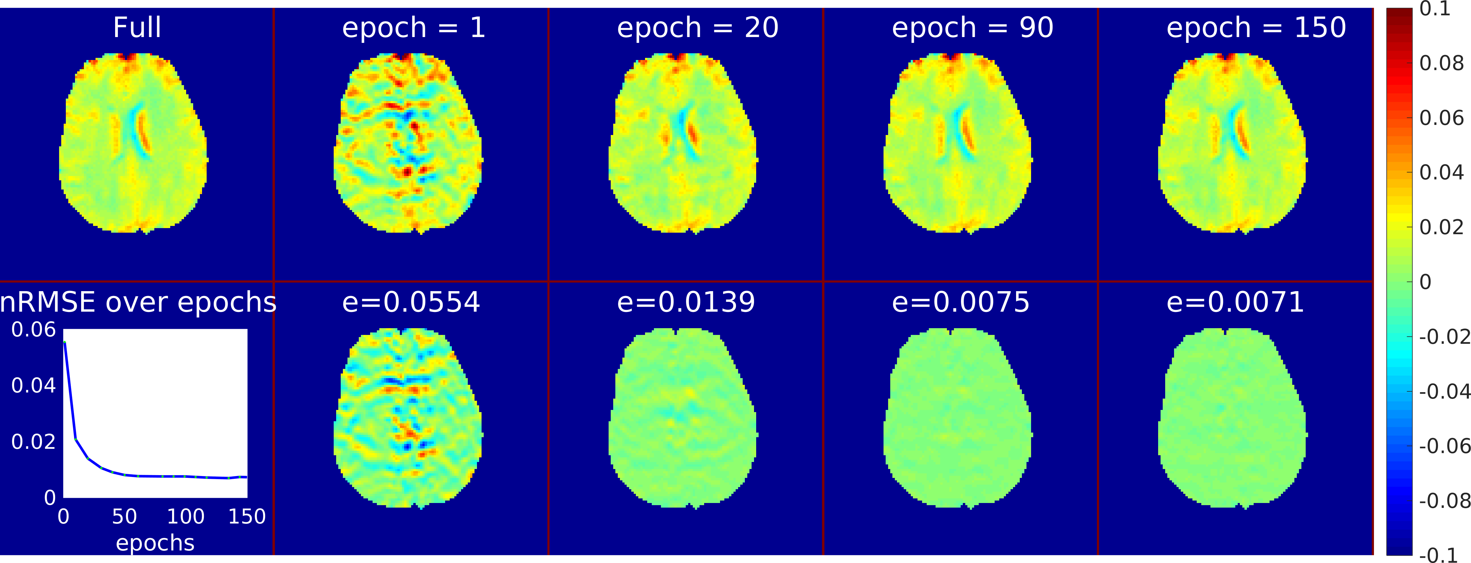
The parallel CRNN (PCRNN) network learns the correlations in spatial-temporal domain and the correlations among iterations. For the CEST application, the temporal domain is replaced by the Z-spectral domain, and PCRNN jointly learns the spatial and Z-spectral features. As shown in Fig.1, the input of the initial iteration is composed of multi-coil undersampled images, and the target of the output is multi-coil fully sampled images. The bidirectional CRNN layers (red bars) were used to learn the spatial-Z correlations, and CRNN layers (yellow bars) were used to learn the dependencies among iterations. Then it projects the extracted features to image domain with convolution layers (green bars). The residual layer (orange summation) allows faster convergece¹². The DC layer (purple bar) constraints the reconstruction image to be consistent to the undersampled k-space data⁹. The reconstruction from the i-th iteration is taken as the new input to the next iteration, which will improve the quality of the input over iterations. All the experiments were performed on a Philips 3T scanner using a 32-channel head coil. CEST images were acquired with a TSE sequence, TR/TE=4200/6.4 ms, slice thickness=4.4 mm, matrix=240x240, FOV=240x240 mm. The saturation RF consisted of 40 pulses each of 49.5 ms duration with 0.5 ms intervals; 31 saturation offsets were recorded between ±7.8ppm with one additional image acquired without saturation for normalization. Data from ten healthy volunteers were collected for training, and the data from three other volunteers were used for testing. For each volunteer, three saturation power levels were tested: 0.7μT, 1.2μT, and 1.6μT. Data augmentation was used for the training data to avoid overfitting. CEST processing used WASSR¹³ for B₀ inhomogeneity correction. MTR_asym­ maps were calculated at 3.5 ppm (Amide Proton Transfer weighted). Software channel compression¹⁴ was performed to combine the 32-coil data into 4 virtual coils. We implemented the learning algorithm with TensorFlow¹⁵. All the computations were performed on a workstation with NVIDIA GTX 1080 Ti GPU. Due to the GPU memory limitation, we resized all of the data to 120x120, and a batch size of 1. Dynamic compressed sensing k-t Sparse SENSE³ was used for performance comparison.

Results and Discussion

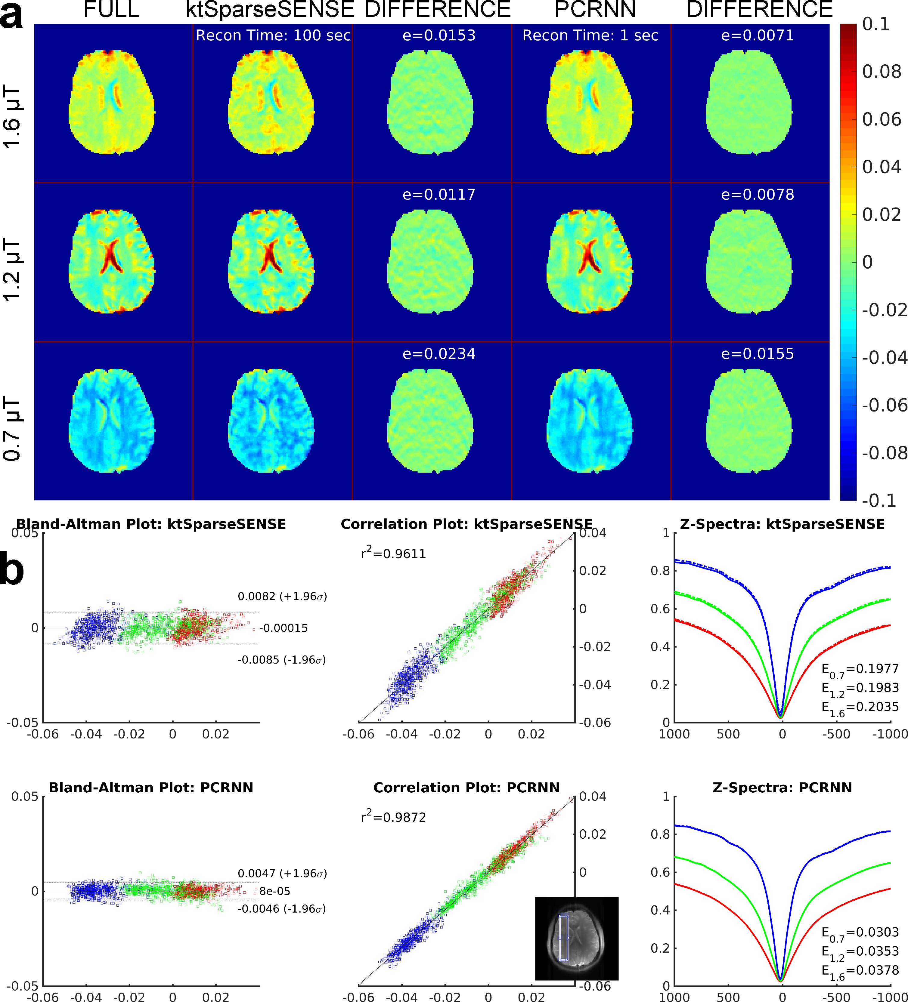
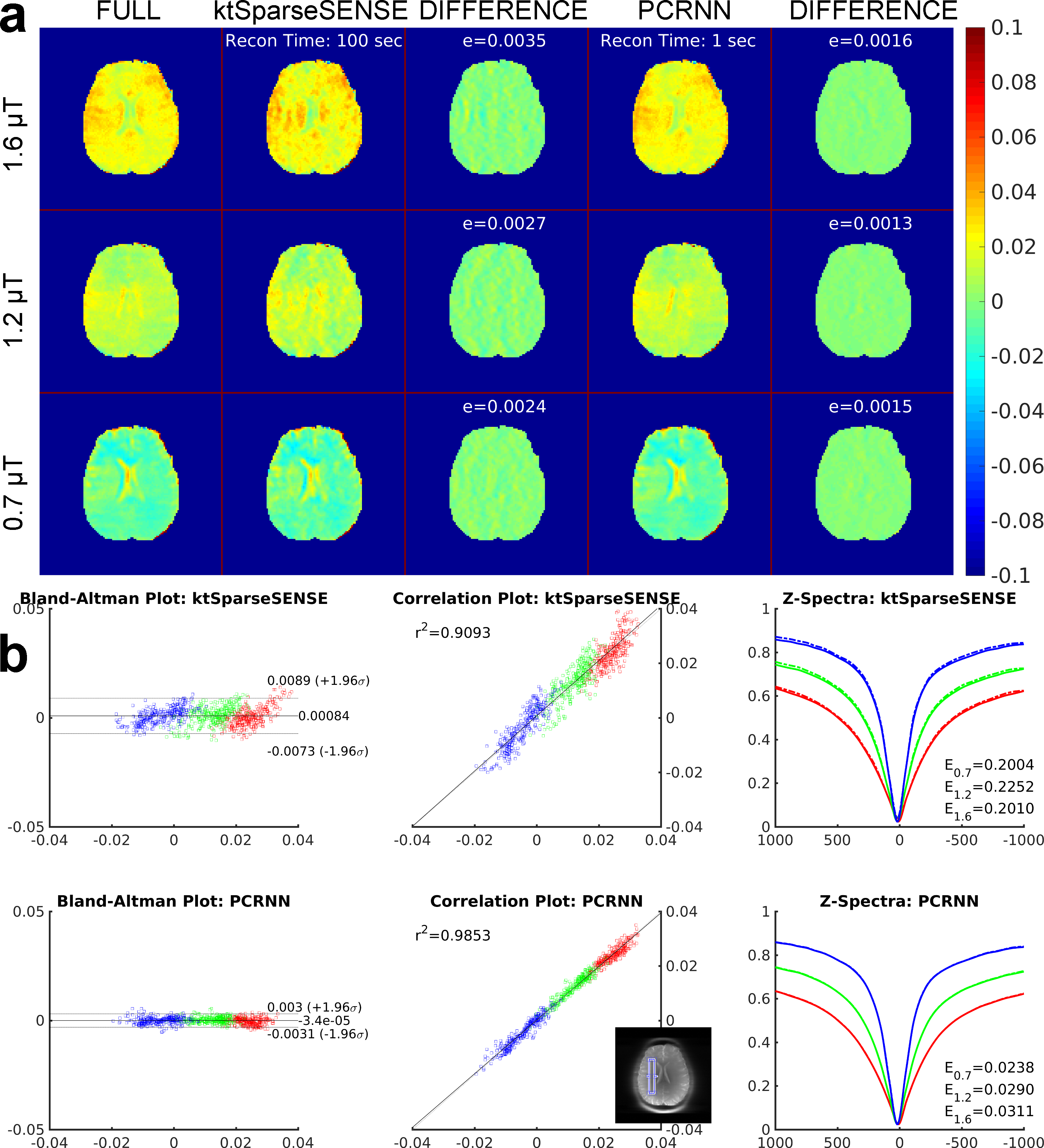
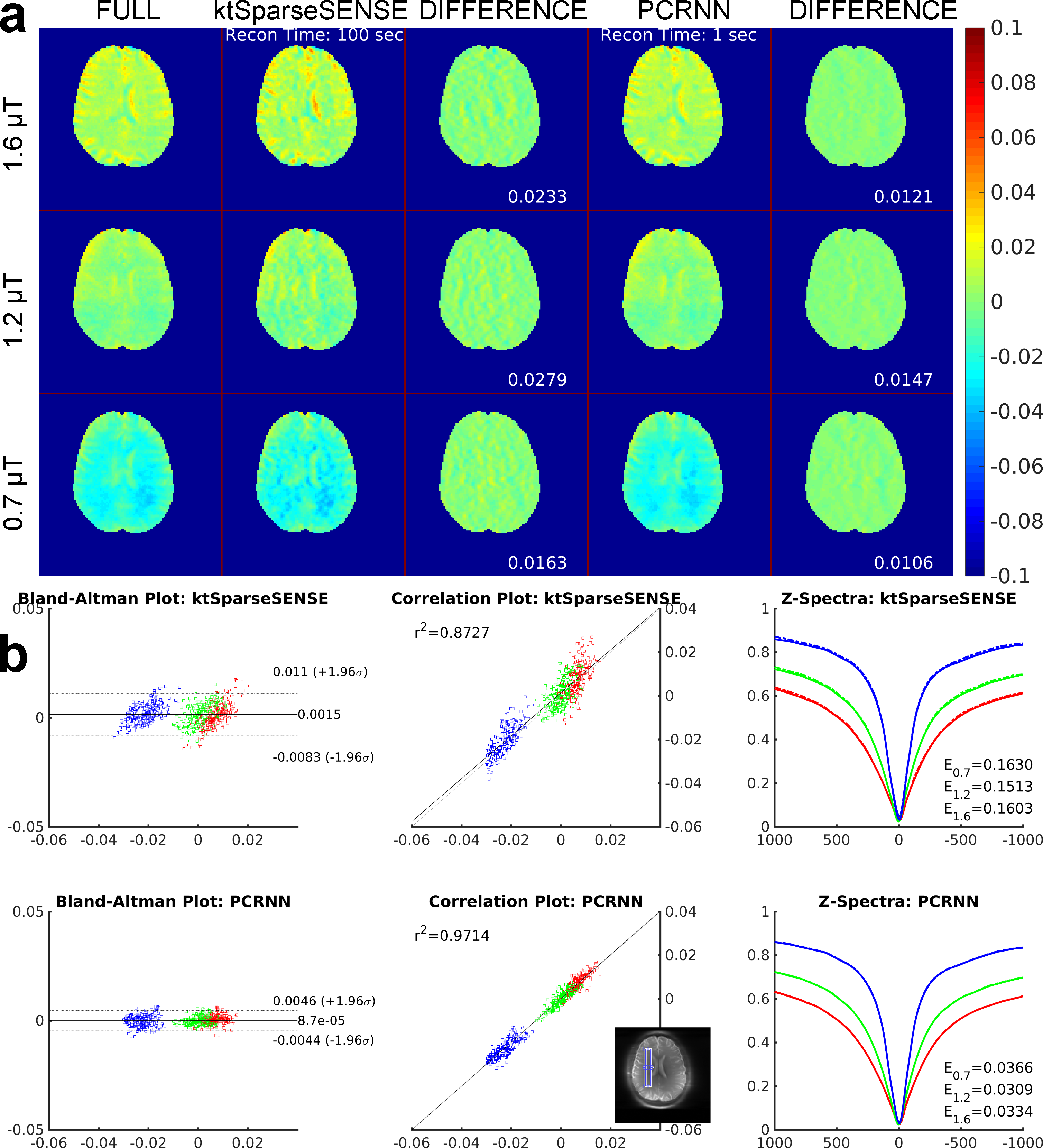
Fig.2-4 compare the results reconstructed using fully sampled, k-t Sparse SENSE and the PCRNN from datasets of the three volunteers. In Fig.2-4 (a), the reconstruction MTR_asym maps and difference images demonstrate that PCRNN can give much better reconstruction quality than k-t Sparse SENSE, the reconstruction error "e" calculated from the normalized square root mean square error⁶ (nRMSE) is shown on the difference maps. Fig.2-4 (b) shows the Bland-Altman plot¹⁶ and correlation plot reconstructed with PCRNN, k-t Sparse SENSE and the fully sampled case for different saturation power in the region of interest (ROI). It is evident that PCRNN leads to higher correlation (r²) with the fully sampled data than k-t Sparse SENSE. Fig.2-4 (b) also shows that PCRNN gives better ROI-averaged Z-spectrum than k-t Sparse SENSE. Importantly, to get these much better quality reconstruction, PCRNN only need around 1 second, which is about one hundred times shorter than k-t Sparse SENSE. Fig.5 shows the testing error of volunteer #1 over training epochs. We can see the testing error decreased fast at first fifty epochs, but does not change much between 120~150 epochs. We evaluated the performance by Cartesian undersampling², and the acceleration factor was R=4. Evaluations at higher acceleration factors (R=6,8,etc) are underway.

Conclusion

We proposed and evaluated a parallel CRNN (PCRNN) learning framework for accelerating CEST imaging. In-vivo human brain results demonstrate that at acceleration rate R=4, the reconstruction quality of PCRNN is much better than k-t Sparse SENSE, while the reconstruction time is one hundred times shorter.

Acknowledgements

This work was supported by the NIH grant R21 EB020245 and by the UTSW Radiology Research fund. We thank Dr. Asghar Hajibeigi for the CEST experimental preparation. We thank Yufei Zhang for image processing and the valuable discussion on the algorithms.