0016

Synthetic MRI through a Deep Neural Network Based Relaxometry and Segmentation

Peng Cao¹, Jing liu¹, Shuyu Tang¹, Andrew Leynes¹, and Peder Larson¹

¹University of California at San Francisco, University of California at San Francisco, San Francisco, CA, United States

Synopsis

This study demonstrated a method for 3D synthetic MRI through a deep neural network Based Relaxometry and Segmentation. Ranges of T1 and T2 values for gray matter, white matter and cerebrospinal fluid (CSF) were used as the prior knowledge. The proposed method can directly generate brain T1 and T2 maps in conjunction with segmentation based bias field correction and synthetic MRI.

Introduction

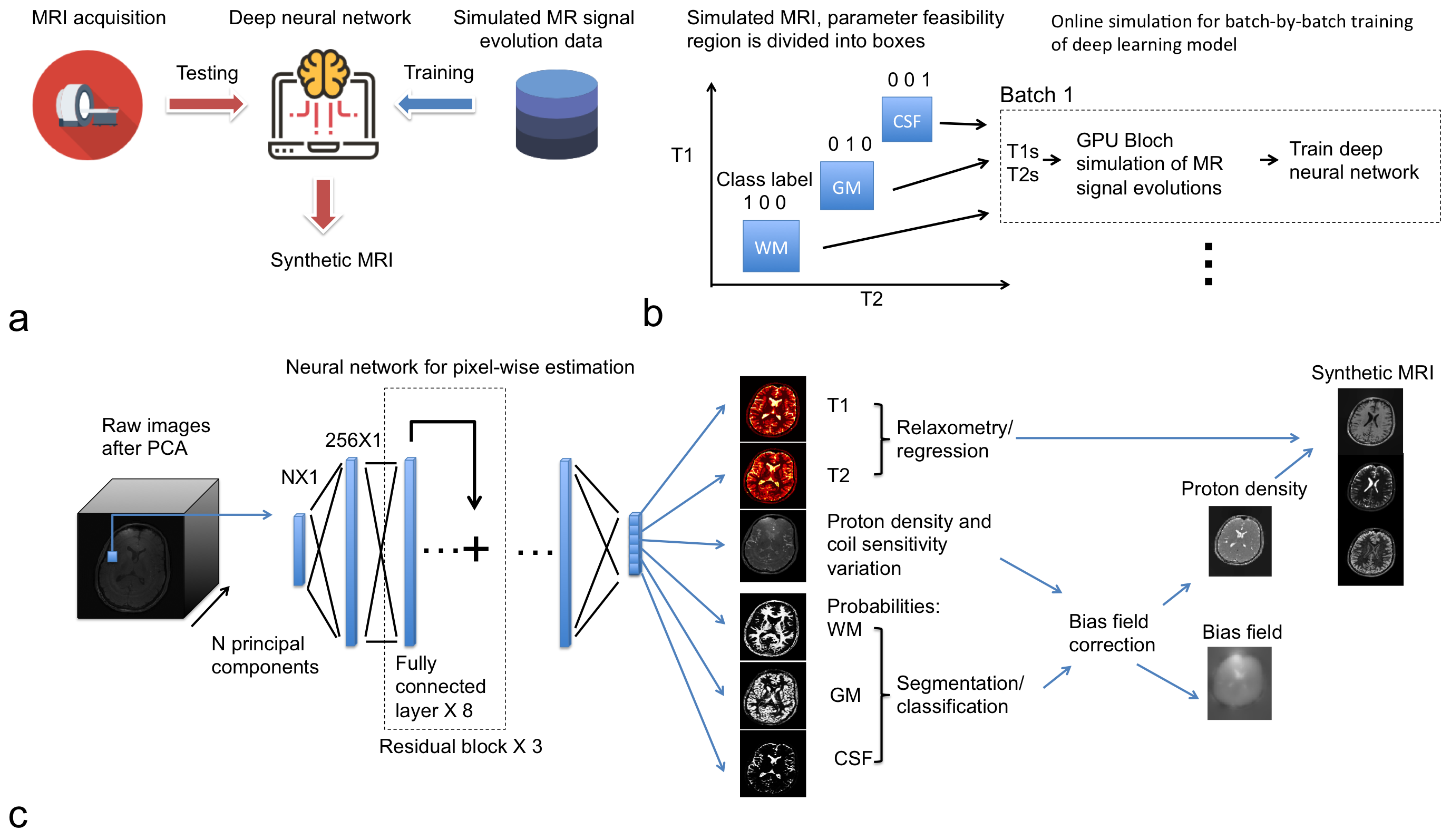
Synthetic MRI through deep neural network based MRI relaxometry and segmentation can allow robust bias field correction and simultaneous multi-contrast MRI, unifying multiple conventional MRI scans. Quantitative MRI allows direct measurement of biophysical parameters of normal and pathological tissues in vivo ^1–4with applications in tissue segmentation/classification ^5–7 and macromolecule quantification ^8–11. A promising method for quantitative MRI is MR fingerprinting (MRF), which uses a dictionary to solve the Bloch equation for deriving T1 and T2 values ¹². Meanwhile, T1 and T2 values in biological tissues are often positively associated with each other ^13,14. We trained a neural network for quantitative MRI measurements to “understand” this association (e.g. a simple box constraints as shown in Fig. 1) with given ranges of T1 and T2 values for gray matter (GM), white matter (WM) and cerebrospinal fluid (CSF). Our results showed that the deep neural network could directly generate 3D T1 and T2 maps in conjunction with the segmentation of gray matter, white matter and CSF and synthetic MRI for in vivo human brain imaging.

Methods

MRI sequence and in vivo data acquisition: An inversion-prepared balanced steady state free precession (bSSFP) sequence was used for acquiring the in vivo dynamic brain images ^15,16. For one volunteer, parameters for IR-bSSFP included FA = 30°, TE/TR=1.5/4.3ms, FOV = 28cm, resolution=1.4×1.1×2.0mm³ and no frequency offsets 15,16. For the other two volunteers, the FOV and image matrix were slightly different from the first one, with FOV = 22cm, resolution=1.4×1.4×2.6mm³, and 2 scans were acquired with no frequency offsets and offset of 1/(2×TR) respectively 15,16. In the IR-bSSFP sequence, after each inversion pulse, data acquisition was set to be 3 s using CIRCUS undersampling strategy^15,16, which allows pseudo-random variable-density sampling with a spiral-like trajectory and golden-ratio profile on the Cartesian ky-kz plane. Images were reconstructed with every 50 TRs at 13 different inversion times (TIs). The acceleration factor was moderate (R=1.3 to 1.6). Neural network design: The deep neural network contained 24 fully connected layers (in Fig. 1) with sigmoid activation, one layer norm and 256 neurons in each layer. The deep neural network was implemented in TensorFlow software package. On-line data simulation in conjunction with neural network training: On-line synthesis of MR signal evolutions and labels was used to train the neural network batch-by-batch (in Fig. 1). Within each batch, uniformly randomized T1 and T2 values, proton densities, binary-labels of tissue/fluid type and varied noise levels were used to simulate MR signal evolutions. The T1 and T2 were uniformly distributed within the ranges: 450<T1<825ms and 25<T2<62.5ms for white matter, 750<T1<1125ms and 55<T2<92.5ms for gray matter, and 2250<T1<3750ms and 125<T2<275ms for CSF, respectively. The cost function for training neural network was designed as mean squared difference between the output of neural network and the known parameters and class labels, and ADAM optimizer was used ¹⁷.

Results

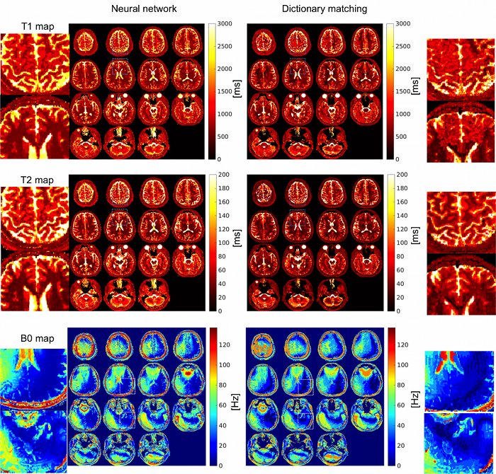
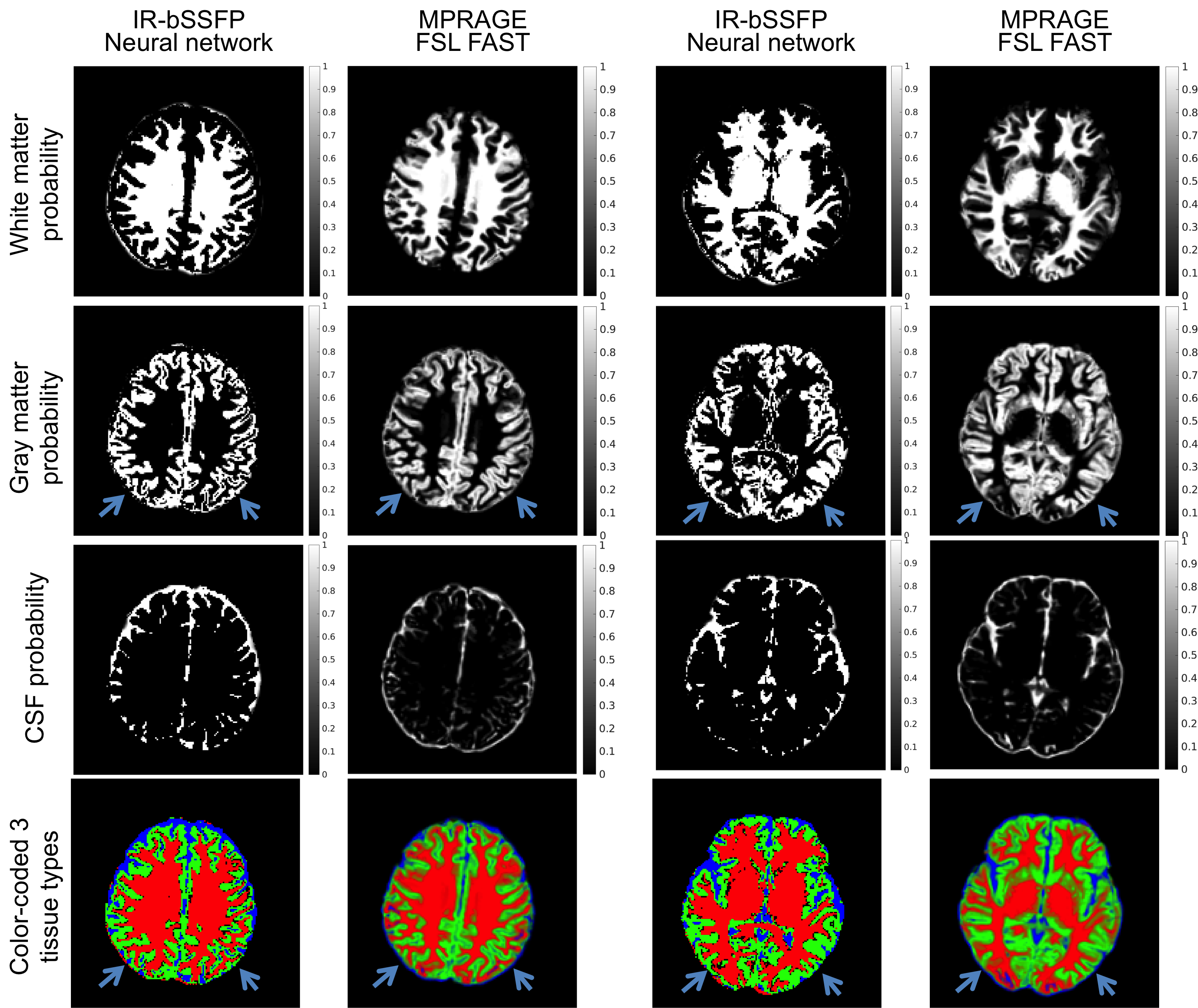
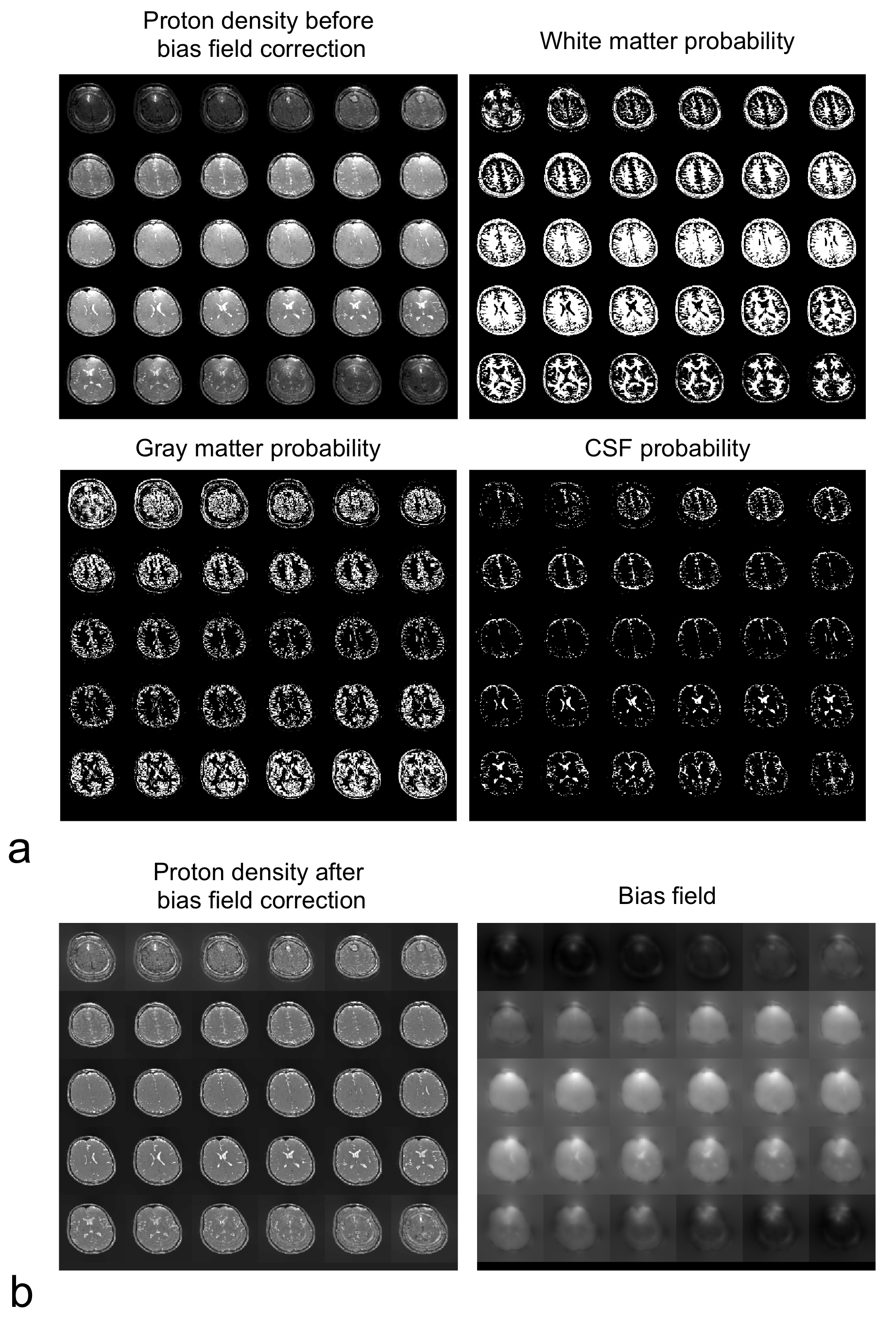
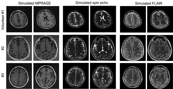
Figure 2 shows the comparison of the quantification results from neural network and dictionary matching. In this study, two IR-bSSFP scans with varied frequency offsets were acquired, which allowed for the estimation of a B0 map in both neural network and dictionary matching methods. The dictionary matching method was vulnerable to scattering artifacts in apparent T1 and T2 maps and quantization/discretization errors in B0 maps, especially in the high B0 variation areas. On the other hand, the deep neural network can produce relatively accurate apparent T1 and T2 maps as well as continuously valued B0 maps. In Figure 3 the neural network segmentation matched the FSL FAST segmentation results in general, with slightly improved gray matter separation in the cortex (arrows in Fig. 3); while FAST is better at some deep brain structures. Figure 4 shows result from bias field correction on the proton density map. In Figure 5, results show that the typical three MRI contrast weighted images, MPRAGE, spin echo, and T2-FLAIR were simulated based on the neural network results.

Discussion

In this study, simultaneous relaxometry and segmentation of in vivo human brain was performed within seconds using a trained deep neural network. The relaxometry and segmentation results from deep neural network were then used in bias field correction and synthesizing the multi-contrast MRI.

Conclusion

In conclusion, the proposed deep neural network method trained with MR signal simulations can directly generate apparent T1 and T2 maps as well as synthetic T1 and T2 weighted images in conjunction with segmentation of gray matter, white matter and CSF.

Acknowledgements

No acknowledgement found.

References

1. Alexander, A. L. et al. Characterization of Cerebral White Matter Properties Using Quantitative Magnetic Resonance Imaging Stains. Brain Connect. 1, 423–446 (2011).

2. Deoni, S. C. L. Magnetic Resonance Relaxation and Quantitative Measurement in the Brain. Methods Mol Biol 711, 65–108 (2011).

3. Laule, C. et al. Magnetic Resonance Imaging of Myelin. Neurotherapeutics 4, 460–484 (2007).

4. Tofts, P. Quantitative MRI of the Brain. Quantitative MRI of the Brain Measuring Changes Caused by Disease (John Wiley & Sons, Ltd, 2003). doi:10.1002/0470869526

5. Chai, J.-W. et al. Quantitative analysis in clinical applications of brain MRI using independent component analysis coupled with support vector machine. J. Magn. Reson. Imaging 32, 24–34 (2010).

6. West, J., Warntjes, J. B. M. & Lundberg, P. Novel whole brain segmentation and volume estimation using quantitative MRI. Eur. Radiol. 22, 998–1007 (2012).

7. West, J., Blystad, I., Engström, M., Warntjes, J. B. M. & Lundberg, P. Application of Quantitative MRI for Brain Tissue Segmentation at 1.5 T and 3.0 T Field Strengths. PLoS One 8, e74795 (2013).

8. Sled, J. G. & Bruce Pike, G. Quantitative imaging of magnetization transfer exchange and relaxation properties in vivo using MRI. Magn. Reson. Med. 46, 923–931 (2001).

9. Yarnykh, V. L. Fast macromolecular proton fraction mapping from a single off-resonance magnetization transfer measurement. Magn. Reson. Med. 68, 166–178 (2012).

10. Yarnykh, V. L. Time-efficient, high-resolution, whole brain three-dimensional macromolecular proton fraction mapping. Magn. Reson. Med. 75, 2100–2106 (2016).

11. Mezer, A. et al. Quantifying the local tissue volume and composition in individual brains with magnetic resonance imaging. Nat. Med. 19, 1667–1672 (2013).

12. Ma, D. et al. Magnetic resonance fingerprinting. Nature 495, 187–192 (2013).

13. Wansapura, J. P., Holland, S. K., Dunn, R. S. & Ball, W. S. NMR relaxation times in the human brain at 3.0 Tesla. J. Magn. Reson. Imaging 9, 531–538 (1999).

14. Wright, P. J. et al. Water proton T1measurements in brain tissue at 7, 3, and 1.5T using IR-EPI, IR-TSE, and MPRAGE: Results and optimization. Magn. Reson. Mater. Physics, Biol. Med. 21, 121–130 (2008).

15. Liu, J. & Saloner, D. Accelerated MRI with CIRcular Cartesian UnderSampling (CIRCUS): a variable density Cartesian sampling strategy for compressed sensing and parallel imaging. Quant Imaging Med Surg 4, 57–67 (2014).

16. Liu, J., Haraldsson, H., Feng, L. & Saloner, D. Free-Breathing Whole Heart CINE Imaging with Inversion Recovery Prepared SSFP Sequence: Feasibility for Myocardium Viability Assessment. ISMRM 22nd Annu. Meet. Exhib. 2410 (2014). doi:10.1038/nprot.2014.167

17. Kingma, D. P. & Ba, J. Adam: A Method for Stochastic Optimization. 2017 IEEE Int. Conf. Consum. Electron. 434–435 (2014). doi:10.1109/ICCE.2017.7889386

Figures

Figure 1 (a) MRI signal synthetic model. The proposed method assumed the feasible parameter space could be divided into boxes that were binary labeled for white matter (WM), gray matter (GM), and cerebrospinal fluid (CSF). (b) A deep neural network was used to perform pixel-wise estimation of T1, T2, B0 (not shown) and proton density/M0 (weighted by coil sensitivity variation) as a regression output, and WM, GM and CSF probabilities as a classification output. The bias field correction, with the tissue segmentation input, was applied to the raw proton density/M0 maps before synthesizing the multi-contrast MRI.

Figure 2 In vivo 3D apparent T1, T2 and B0 estimation using both the proposed deep neural network and dictionary matching. Data was acquired with 3D IR-bSSFP, 30 inversion times, and 2 different frequency offsets at 0 and 1/(2×TR). The dictionary matching was vulnerable to scattering artifacts in T1 and T2 maps and quantization/discretization errors in B0 maps. On the other hand, the deep neural network outputs appear more accurate relative to brain anatomy as well as continuous (or piecewise continuous) T1, T2 and B0 values.

Figure 3 Whole brain segmentations comparisons between the direct output of neural network and FSL FAST (same study as Fig. 4). In general, the neural network based segmentation matched FSL FAST segmentation results. The neural network showed robustness in segmenting gray matter in the cortex (arrows) but did not correctly segment the putamen on this slice. The skull stripping was performed using the BET algorithm in FSL.

Figure 4 (a) Typical inputs for the bias field correction: proton density/M0 map (with the coil sensitivity variation and aliasing artifacts), white matter, gray matter, and CSF probabilities. (b) Effective bias field correction was achieved with the use of brain segmentations.

Figure 5 Simulated MPRAGE images (inversion time = 1500 ms, TR = 3500 ms), spin echo (TE = 80 ms) and T2-FLAIR images (TE/TR = 80/3500 ms, inversion time = 1500 ms), from the T1, T2 and proton density/M0 results of neural network. The bias field correction, with the tissue segmentation input, was applied to the raw proton density/M0 maps before the simulation.

Proc. Intl. Soc. Mag. Reson. Med. 27 (2019)

0016